Exercise 8 – RS Part 2
Explore imagery – Spatial resolution
By Madeline Wrable and Delphine Khanna*
One important characteristic of imagery data is its resolution. There are four types of resolution: spatial, temporal, spectral, and radiometric. In this tutorial, you’ll learn about spatial resolution.
You’ll become familiar with the concept of spatial resolution and examine satellite imagery of different spatial resolutions in ArcGIS Pro. Your exploration will focus on the region of Pembamoto, Tanzania, where an innovative regreening project is taking place. You’ll also apply your knowledge of spatial resolution to change the cell size of imagery using resampling and verify your results using the measuring tools.
Objectives:
Learn about spatial resolution and compare four different satellite imagery datasets. Practice changing the cell size of imagery using the Resample tool and verify pixel sizes using the Measure tool.
Outline
| Task 1 – Visualize spatial resolution – Learn about spatial resolution and compare the spatial resolution of four satellite images. | 15 minutes |
| Task 2 – Identify the cell size of an image – Learn how to find the spatial resolution of an image by examining its properties or by measuring its cells. | 5 minutes |
| Task 3 – (Optional) Change the spatial resolution of an image – Learn about changing spatial resolution and resampling imagery to a larger cell size. | 10 minutes (Optional) |
Task 1 – Visualize spatial resolution
First, you’ll learn about the concept of spatial resolution. Then, you’ll explore satellite imagery of varying spatial resolutions.
A- Learn about spatial resolution
Imagery can be collected by aircraft, drones, satellites, and ground-based sensors, and by scanning historical maps. It is stored in raster format, which represents information as a grid of cells (or pixels).

Spatial resolution (also known as pixel size or cell size) is the dimension of the area covered on the ground and represented by a single cell. If a dataset is said to have a 10-meter spatial resolution, it indicates the length of one side of a cell, meaning that each cell represents a 10-meter by 10-meter square (100m2 area) on the ground.
Spatial resolution affects the level of detail represented in an image. If the cells are of a smaller size, the spatial resolution is said to be higher, and more details of the real world can be captured in the raster. For example, in the following graphic, the raster on the left has a higher spatial resolution than the raster on the right.

Note: Some (large) pixel sizes force multiple features within a cell to be summarized by a single value.
Higher spatial resolution requires more computer storage and takes more time to process and analyze. It can also require purchase of commercial data. When choosing a spatial resolution for the raster data in a project, you should ensure that it is:
- High enough to capture the features of interest to your project (for example, do you need to see the mountains, the rivers, the fields, the roads, and so on?)
- Low enough to minimize computer storage, processing time, and potential associated costs.
For satellite imagery, spatial resolution can commonly vary across sensors. Some examples of spatial resolutions include 1000m, 500m, 250m (MODIS), 90m, 60m, 30m (ASTER), 30m (Landsat), 10m (Sentinel), 5-3m (PlanetScope), or 0.5m (SkySat). For imagery captured from aircrafts or drones, the spatial resolution can be much higher, ranging from 1m (NAIP) to 1cm (drones) or even less. This tutorial focuses on satellite imagery.
NOTE: This part uses the extension Spatial Analyst, make sure it’s activated as indicated at the beginning of exercise 7 (task 0)
B- Explore Pembamoto at the regional scale
Next, you’ll explore satellite imagery and its spatial resolution in ArcGIS Pro, with a focus on the area of Pembamoto, Tanzania. You’ll examine imagery that can efficiently depict the larger Pembamoto region. First, you’ll set up the ArcGIS Pro project.
1- Copy the corresponding data (\ex8) from the class folder into your working folder. Go to your working folder and launch the project called Pembamoto.aprx in \ex8\Pembamoto folder
Confirm that the Pembamoto region map is selected on top of the map window.
The map displays the default topographic base map and is focused on Tanzania. A small red rectangle, east of Dodoma, shows the general region of interest for this tutorial.

2- In the Contents pane, right-click Region_of_interest and choose Zoom To Layer.

The map updates, revealing an imagery layer named Landsat9 – 01/28/2023 – 30m – region.

This is a Landsat 9 satellite image that was captured on January 28, 2023, and was clipped to the size of the red rectangle. Landsat 9 images have a 30-meter spatial resolution, which makes them effective at representing larger extents, such as an entire region, without using up too much storage space.
Note: Landsat 9 is a satellite mission from USGS and NASA launched in 2021. It produces imagery with 11 spectral bands, most of them with a 30-meter spatial resolution. The images cover the entire planet, and every place on Earth is captured every 16 days (or every 8 days if combined with Landsat 8 images). Landsat is the longest-running satellite imagery acquisition program, providing five decades of continuous earth observation data. Landsat images are freely available.
Learn how to download your own Landsat imagery (Optional).
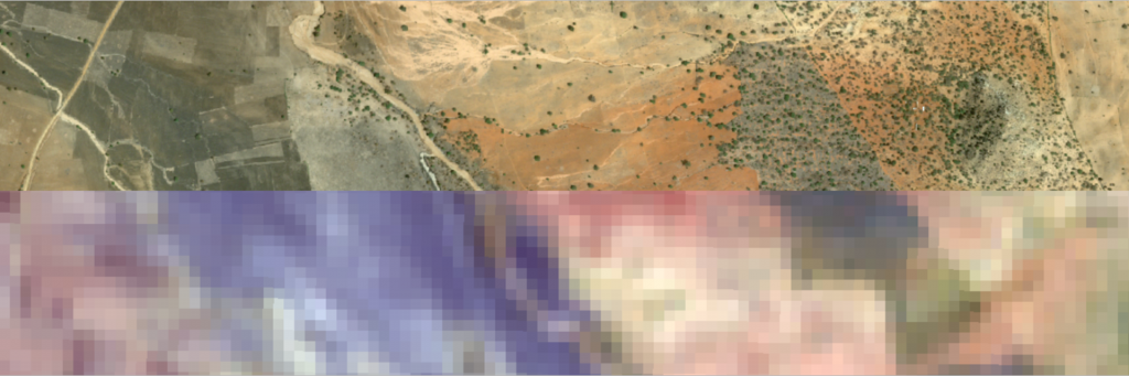
3- Observe the imagery.
Can you identify different land cover types in the region? (Zoom in & out and pan around the study area)
- Arid areas with mostly bare earth and sparse vegetation (light pink and dark pink tones)
- Mountainous areas with some vegetation (rugged areas in greenish tones)
- Heavily vegetated valleys (dark green)

Landsat imagery depicts (1) arid areas, (2) mountainous areas with some vegetation, and (3) heavily vegetated valleys.
4- Use the mouse wheel to zoom in until the image becomes pixelated and you can see the individual cells.

With a 30-meter cell size, Landsat 9 images do not allow you to identify small features on the ground, such as individual houses or trees.
5- Zoom out and back in to different areas of the image to examine it further.
Overall, Landsat images are ideal to identify and monitor regional phenomena, such as desertification, urban expansion, or other land cover change trends.
C – Compare spatial resolutions
Now that you have become familiar with the larger Tanzania region, you’ll zoom in to discover the vegetation restoration project taking place in the Pembamoto locality. The NGO Justdiggit, which seeks to fight global warming by regreening Africa, worked with the local Pembamoto community to dig a series of “bunds” (semicircular shaped pits) that help the soil capture rainwater. Thanks to the creation of these bunds, the site, previously arid and dry, showed dramatic vegetation growth in just a few years.


NOTE: To learn more about this project, see Seeing African Restoration From Space, Northern Tanzania Work, and the Quantifiable impact: monitoring landscape restoration from space. A regreening case study in Tanzania research article.
You’ll examine the site of the Pembamoto regreening project using satellite images with different spatial resolutions, captured between December 2022 and January 2023. First, you’ll switch to the next map.
1- Click the Regreening project map tab.

The map shows the same general Pembamoto region you examined earlier. A small red rectangle indicates the much smaller area of interest (AOI) where the regreening project is located.

2- In the Contents pane, right-click Pembamoto_AOI and choose Zoom To Layer.

In the Contents pane, there are four imagery layers, currently turned off.

The name of each image lists the image type, the date it was captured, and the spatial resolution. These images have been clipped to the AOI dimensions, and their spatial resolution varies from 30 to 0.5 meters. You’ll turn on the layers from the lowest to highest spatial resolution to compare them.
3- Check the box next to the Landsat9 – 01/28/2023 – 30m layer to turn it on.

The image appears on the map.

This is the same Landsat image as the one you saw earlier, but now clipped to fit the smaller AOI. Unsurprisingly, at this larger scale, the Landsat image appears somewhat pixelated. However, it still allows you to clearly see the regreening project area, which appears in dark green tones. The unvegetated grounds surrounding it appear in pinkish or bluish tones depending on soil types and underlying geologic formations.

4- In the Contents pane, turn on the Sentinel2 – 12/09/2022 – 10m layer.

The image appears on the map.

This is a Sentinel-2 satellite image that was captured on December 9, 2022. Sentinel-2 images have a spatial resolution up to 10 meters, which makes them quite versatile, as they can still be used for region-level display and analysis but can also show more detailed features on the ground. At the current scale, the image is not pixelated and shows the regreening project area very clearly. You can also identify other features, such as a few mountains in the north, some agricultural fields in the southeast, and several roads. East of the mountains, a white cloud was captured. Can you spot the cloud’s shadow?
NOTE: Sentinel-2 is a satellite mission from the European Space Agency. It was launched in 2015 and produces imagery with 13 spectral bands, several of which have a 10-meter resolution. The images cover the entire earth and every place on earth is captured at least every 5 days.Sentinel-2 images are freely available and can be downloaded through the Copernicus Data Space Ecosystem.
5- In the Contents pane, turn on the PlanetScope – 01/01/2023 – 3m layer.

This is a PlanetScope satellite image that was captured on January 1, 2023. PlanetScope images have a 3-meter spatial resolution, depicting many detailed features on the ground. Imagery with that type of spatial resolution is frequently used for feature-scale analysis and includes agriculture, archeology, infrastructure, and forestry applications.
In the image, you can see many of the same features as previously, but they appear more detailed. Darker brown fields have appeared in several areas, suggesting that late December was a time of active tilling (preparing and cultivating land for crops) or other agricultural activities.
NOTE: PlanetScope images are produced by the private company Planet Labs. PlanetScope is a collection of over 180 satellites that was deployed from 2014 onward and produces imagery with a 3-meter resolution and up to 8 spectral bands. The images cover nearly the entire landmass of Earth, and each location is captured almost daily.
6- In the Contents pane, turn on the SkySat – 12/13/22 – 0.5m layer.

This is a SkySat satellite image that was captured on December 13, 2022. SkySat images have a 0.5-meter spatial resolution, depicting features on the ground with a high level of detail. Imagery with that type of spatial resolution is frequently used for precision mapping, 3D city modeling, or precision agriculture.
In the image, you can see many details, such as individual trees and bushes, and subtle nuances on the ground.
NOTE: SkySat images are produced by he private company Planet Labs. SkySat is a collection of about 20 satellites that was deployed from 2013 onward and produces imagery with a 0.5-meter resolution and 4 spectral bands. SkySat satellites can be actively maneuvered to capture imagery from any location on Earth.
You have now reviewed all of the images provided in this project.
7- Explore the images further by turning them on and off and zooming in and out with the mouse wheel.
Tip: Whichever layers are on top will block your sight of the layers below, so turn them on or off accordingly.
D- Explore cell sizes and spatial extents
You’ll continue your exploration of spatial resolution by zooming in to specific areas around the Pembamoto regreening site using bookmarks. You’ll also compare the extent of the original images.
1- On the ribbon, click the Map tab. In the Navigate group, click Bookmarks.

To better understand the notion of cell size, you’ll zoom in a level of detail where you see individual cells.
2- In the list of bookmarks, choose Cells.

3- In the Contents pane, turn off all four imagery layers (the Landsat-9, Sentinel-2, PlanetScope, and SkySat layers) and turn them back on one by one.

(1) Landsat-9, (2) Sentinel-2, (3) PlanetScope, and (4) SkySat images.
The cell sizes vary drastically. How many cells does the current extent contain for each imagery type? It only contains a few Landsat 9 cells, about 60 Sentinel-2 cells, a few hundred PlanetScope cells, and thousands of SkySat cells.
4- On the ribbon, on the Map tab, click Bookmarks and choose Roads and fields.

The map zooms in to an area on the east side of the AOI.
5- In the Contents pane, turn off all four imagery layers and turn them back on one by one.
 (
(
1) Landsat-9, (2) Sentinel-2, (3) PlanetScope, and (4) SkySat images.
If you wanted to choose imagery that requires as little storage as possible but that allows you to distinguish the main roads, which of the four images would you choose? What if you needed to distinguish secondary roads or dirt tracks? Agricultural fields? Houses? Individual trees and bushes?
Question 6. You can use Landsat images to to distinguish houses and individual trees and bushes.
True – False
6- Now zoom to the Town bookmark and make similar observations.
While the four imagery layers were clipped to fit the AOI boundaries, the original images captured by the different satellites were significantly larger.
The following illustration represents every image in its full original extent; the Pembamoto AOI is represented as a small red rectangle in the lower left quadrant.
What do you observe about the relative sizes of these images? For Landsat 9, because the cell size is so large, a single image can capture a very large extent. As you move to imagery with smaller and smaller cell sizes, a single image can capture a smaller and smaller extent. This is a general trend, although the exact number of cells per image depends on each sensor’s technical specifications.
Question 7. For the same extent Landsat images require the least amount of storage.
True – False
In this part of the tutorial, you became familiar with essential spatial resolution concepts and compared satellite images with different spatial resolutions. You explored the Pembamoto area and learned about an innovative regreening project taking place there. One takeaway is that there is a trade-off between the greater level of detail that high spatial resolution imagery provides and the lower storage space and processing time that low spatial resolution imagery requires. You should take this trade-off into account when choosing imagery for a project.
The AOI polygon in the Regreening Project map measures about 5 kilometers on the side (a little longer in east-west direction; verify this number yourself). The 4 images used here have been clipped (Extract by Mask) to this AOI but because of the different resolutions each one will have different numbers of pixels in the same area.
Question 8. What is the number of pixels of each image within the AOI?
(Hint 1: get the properties)
Landsat 9 ______
Sentinel 2 ______
Planetscope ______
Skysat _______
Task 2 – Identify the cell size of an image
Every image you encountered in this workflow had its spatial resolution listed in its name. However, when you receive an imagery dataset in real life, you may not know its spatial resolution. Next, you’ll learn how to find that information.
A- Find the cell size in the image properties
The standard way of finding the cell size of an image is by examining its properties.
1- Ensure that the Resampling map tab is selected.

2- In the Contents pane, right-click PlanetScope_01012023_3m and choose Properties.

3- In the Properties pane, click the Source tab, expand the Raster Information section, and locate the Cell Size X and Cell Size Y fields.

The Cell Size X and Cell Size Y fields each have a value of about 3. This means that each cell represents a square of 3 by 3 meters on the ground. You might not be sure whether the unit of measurement is meters. You can find this information under the Spatial Reference section.
4- Expand Spatial Reference and locate the Linear Unit field.

That section contains information about the image projection and coordinate system. The Projected Coordinate System value is WGS 1984 UTM Zone 37S, while the Linear Unit value is Meters. This confirms that the cell size is expressed in meters. You now know that your PlanetScope image has a cell size of 3 meters.
5- Use what you learned to check the cell size of the PlanetScope_01012023_10m layer (in the Regreening project map).
B- Measure imagery cells
Finally, you’ll learn how to measure the cells of an image yourself. While looking in the imagery properties is the most common method, measuring the cells yourself is a good way of further demystifying the concept of cell size.
1- In the Resampling map, ensure that PlanetScope-01/01/2023_10m and PlanetScope-01/01/2023_3m are turned on.

NOTE: The file names, as you can see, do not contain backslashes as this is a “reserved” character in Windows. The instructions have backslashes to make things easier to read. We could rename the theme names in the CP if we wanted, like in the other tabs
PlanetScope-01/01/2023_10m is displaying on top, so you’ll measure it first.
2- If necessary, on the ribbon, on the Map tab, click Bookmarks and choose the Cells bookmark.

3- On the ribbon, on the Map tab, in the Inquiry section, click Measure.

On the map, the Measure distance window appears, as well as the measuring pointer.
4- Click two sides of a cell to measure its width.

The cell is approximately 10 meters wide.
5- In the Measure Distance window, click the Clear Results button.

6- In the Contents pane, turn off the PlanetScope-01/01/2023_10m layer.

On the map, the PlanetScope-01/01/2023_3m image appears.
7- Click two sides of a cell to measure its width. It is approximately 3 meters wide.

Question 9. What is the diagonal distance of one cell in PlanetScope-01/01/2023_10m layer?
(Hint: you can also use Pythagoras theorem to calculate the length of the hypotenuse)
8- When you are finished measuring, on the ribbon, on the Map tab, click the Explore button to close the measuring mode.

In this tutorial, you became familiar with essential spatial resolution concepts. You learned to visually distinguish imagery with higher or lower spatial resolution and to select the spatial resolution best adapted to your project. You learned how you can change the spatial resolution of an image and became familiar with several resampling methods. Finally, you learned how to find the spatial resolution of an image either by looking in its properties or by measuring its cells directly.
NOTE: Work on Task 3 (it’s very short) to learn how PlanetScope-01/01/2023_10m was created from the 3m layer using a method called Resampling.
Go to Task 3 (Optional)
Go to start page Mapping & Spatial Analysis
Source:
This tutorial was originally developed by the Esri Tutorials Team.
You can find the official maintained version at this location
https://learn.arcgis.com/en/projects/explore-imagery-spatial-resolution/
You can find other tutorials in the tutorial gallery [https://learn.arcgis.com/en/gallery/].