Vector Analysis (DB Query)
Contents
- Part 1: Tutorial – Database Queries and Multi-Criteria Evaluation
- Objective: Learn vector analysis while finding a suitable town to move to in New Jersey
- Part 2: Case Study – Practice with Database Queries and Multi-Criteria Evaluation
- Objective: Practice the skills from Part 1 while finding a county to move to in Massachusetts
Part 1: Tutorial: Database Queries and Multi-Criteria Evaluation
For this part of the exercise, you will ask (query) a series of spatial and non-spatial questions to find a town you want to live in, using vector data from the Hackensack River watershed at the northeast corner of New Jersey. You will be looking for a town in Bergen County with a small but not shrinking population with a large stream or river running through it. Additionally, you only want to live on roads that are close to a public school. Your final goal is to figure out which of the towns that meet your criteria has the greatest length of suitable roads—a good place for you to visit with the realtor.
Index of part 1
- Preliminary tasks
- DATABASE QUERY BY LOCATION
- QUERY BY SINGLE AND MULTIPLE ATTRIBUTE
- ALGEBRA
- SPATIAL ANALYSIS
Preliminary tasks
- Once you have copied the folder \ex4, from the N: drive to your X: drive, launch ArcGIS Pro and make a new project using the \ex4 folder as your working folder (don’t create a new folder).
- Add all the themes inside NJData.gdb to the map.
The geodatabase (NJData.gdb) contains the following feature classes (themes):
- Municip (polygon) – political units/municipalities in New Jersey (boroughs, cities, townships, villages). The outlines of the “outer” municipalities are not complete, as they have been clipped to the shape of the Hackensack river watershed.
- Public (point) – public buildings/properties (parks, schools, town halls, churches, etc.)
- Roads (line)
- Streams (line)
You will use these themes to find municipalities that meet the following criteria:
- Low population (less than 30,000 people in the year 1990)
- In Bergen County
- Low population loss (loss of no more than 200 people between 1980 and 1990)
- Intersected by a large stream or river
Then, you will figure out which of the towns has the greatest length of roads within 2000 feet of a public school.
DATABASE QUERY BY LOCATION
Database query by location in ArcGIS is really a query by feature. When doing a query by location in ArcGIS Pro, we ask the question: “For the feature at this location, what are the associated attributes?” (The attribute table will also be referred to as the database associated with a particular theme). We can query by a single feature (location) or by several at once.
Task 1: Query by single features
Explore the layers and get familiar with them. You can use the Explore cursor to query by a single location or feature. Let’s find the name of the stream at the very top of the study area.
- Display the theme Streams on its own or easily visible on top of another theme. Display it with a graduated symbol using the column ORDER_ as the Field value.
- Get the EXPLORE cursor and left click the stream at the top of the map (it runs almost straight north south). You need to be very precise where to click to get it!
The EXPLORE results pop-up dialog box that appears and shows the name of the stream, Bear Brook, as well as all of the other associated attributes for that one feature (if you don’t get the name of the stream, ArcGIS Pro might be giving you the result of another layer in the current map. Turn off all layers but STREAMS in the dialog window, if necessary).
- Now make other themes visible and use the EXPLORE tool to explore the attributes of different features.
Question 1 – What is the name of the northern-most municipality?
Question 2 – And what county is it in?
Task 2: Query by multiple features
The EXPLORE tool lets you examine all of the attributes associated with a particular feature, one feature at a time. However, you may want to view the entire database associated with a theme, and you may want to query more than one feature at a time.
- Display only the Public theme.
- Open the attribute table associated with PUBLIC by right clicking the theme name and selecting “Attribute Table”.
NOTE: When you open more than one attribute table at a time, ArcGIS Pro uses a “tabbed” interface. Look for the tabs at the top of the table window. - Scroll sideways through the table to see all of the attributes (arranged in columns or fields) for each feature (arranged in rows also called records).
- The TABLE window should be automatically docked at the bottom or sides of ArcGIS Pro. If not, arrange the TABLE window such that you can also see the map behind.

- Click the SELECT FEATURE button from the Select group of the Map tab in the ribbon interface (white arrow with a blue and white box).
- Move the mouse pointer into the map and select features by either clicking on individual features or drawing a box to select several features at once, or clicking multiple features while holding the Shift key.
- Notice that the selected features turn light blue in the map (for points and lines. If the selected feature were a polygon only the outline will turn blue) and that the records in the attribute table, are associated with those features, also turn blue (make sure to scroll down to see all selected records).

- Click on any empty space to deselect, or go to the Selection group in the Map tab and click the white box to clear the selection.
QUERY BY SINGLE AND MULTIPLE ATTRIBUTE
The methods you have just learned are valuable for some situations—when you want to learn about a particular stream or town, for example. However, think of our goal: it would be nearly impossible to find the best town to visit, according to our criteria, with just this query by location tool. Fortunately, there are other methods.
In addition to query by location, we can also query by attribute. When querying by attribute in ArcGIS Pro we ask, “What features have a particular attribute or set of attributes?” We can build a query that will select from an attribute table all records that have a particular attribute or set of attributes. Both single attribute and multiple attribute queries can be “built” using the “Select by Attribute” option in the Selection group of the Map tab.
Let’s begin by finding towns with a population of less than 30,000—our first criterion.
Task 3: Query by Single Attribute
Now we will identify all municipalities that have low populations. We’ll build a query that selects from the table all records where the value in the field representing population (in 1990) is less than 30,000. These records are associated with individual municipalities/features on our map.
- Display just the Municip theme. If you see only one section of the map, right click on the theme name and select “Zoom to Layer” to see the whole picture.
- Study the attribute table of this theme. Examine the different columns/properties. Can you tell what they are?
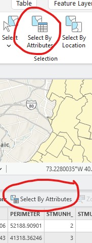
- Make sure there are no polygons selected, and then in the Selection group of the Map tab (or on top of the attribute table) click on “Select by Attributes”.
- Select the theme Municip in the “Input Rows” field.
- Select “New Selection” in the “Selection Type” field.
You will now write an equation that will query (also called “filtering”) the database to select only those records of interest (i.e. where the population in 1990 is less than 30000).
- To do this, first click on “New expression” in the middle of the Select “By Attributes” window to open the query builder.
- You can now do the selection by choosing values from the drop-down menus to construct the ”where” clause.
- Next to the word “Where” click on the drop-down menu of the first box, which contains fields/attribute values for the Municip layer, and select POP90 (POP90 is the field/attribute containing values representing population in 1990 for each municipality).
- In the second box select “is less than” from the drop-down menu.
- In the third/last box type in the number 30000
- Click “Apply” and close the selection window
You just created a SQL (Structured Query Language) statement that looks like this: “POP90” < 30000. This is a standard way of working with Database Management software (DMS). ArcGIS Pro just made it easier for you to do it.
- Notice that the selected features where population is less than 30,000 have a blue outline in the map AND in the attribute table (open the table if it’s not still open).
- In the lower part of the attribute table there are two buttons side by side on the left of where it shows “# out of # selected”. Right now, the left button which means “Show All Records” should be depressed. Press the right button, which means “Show Selected Records.” (As long as ArcGIS Pro is active, hovering the cursor over the icons will show words that describe their function).
Question 3 – How many municipalities have populations less than 30,000? (Hint: see the numbers at the bottom of the table)
Question 4 – Union City is in the selected set. True – False
Task 4: Query by Multiple Attribute
Population size is not your only concern, however. You also want to make sure you are only including towns in Bergen County. Therefore, you need to perform a multiple attribute query to identify municipalities that are both small (population under 30,000) and in Bergen County. This type of query can also be built using the Select by Attribute function.
- First, push the “Show all records” button at the bottom of the attribute table.
- Then deselect the currently selected features by right clicking on the theme’s name (in the CP) and choosing SELECTION/Clear Selection.
- With both the Municip theme and table showing, from the Map tab go to the Selection group and click on “Select by Attributes”.
- READ BEFORE DOING
- Make sure that Municip is selected as Input Rows
- Click on “New expression” and enter the following operation: POP90 is less than 30000 (just like you did above).
- Then, click on Add Clause . Notice there are 4 drop down boxes in this clause.
- In the first drop down box, click the drop-down arrow and select “And” (“And” joins the two clauses of the query together and signifies that you are going to select municipalities that have a small population AND are located in Bergen county at the same time)
- In the next 3 boxes enter COUNTY is equal to BERGEN. NOTE: In the last drop-down box, don’t type BERGEN out—it’s always safer to use the drop down menu in this box whenever possible when writing expressions.
- Then click “Apply” and close the selection window.
Question 5 – How many municipalities have you selected this time?
You have to be careful where you click once you have made a selection! Clicking on the map or in the table may erase your selection. If this happens, you will have to repeat the operation. To avoid this problem, and to save your work for later, it is often best to make a permanent copy of your selection.
- To do this, right click on the Municip name in the CP, and go to “Data\Export Features”. This will save the objects (features) that are selected as a new theme.
- Make sure Input Features is Municip
- Output Location should be your project default (e.g. ex4.gdb)
- Name the output “Selected_Municip” (notice the underscore between words. The software doesn’t like spaces inside a GeoDB)
- The new theme will show in the CP. Open its attribute table and make sure that only the selected municipalities were exported (the same number as Question 5, above)
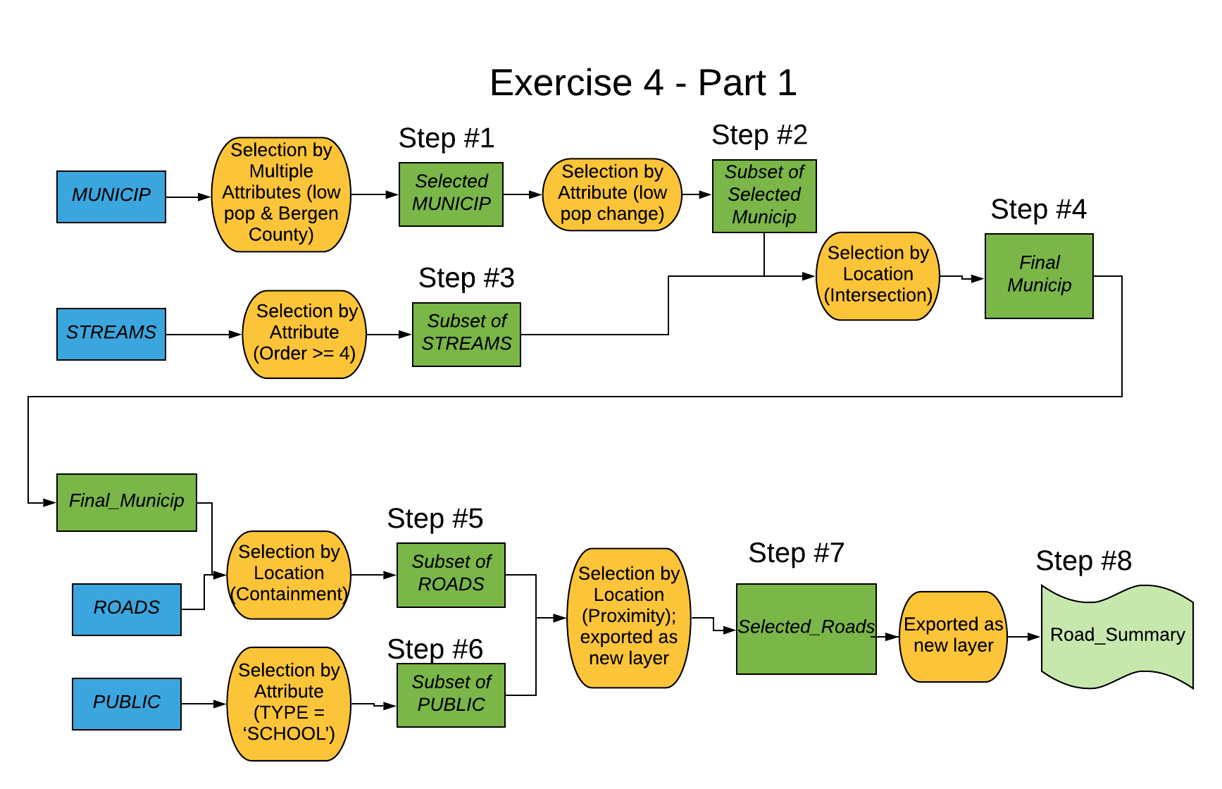
Step #1 in cartographic model
MAP ALGEBRA
Map algebra refers to the calculation of new data from existing data. New attributes (such as changes in population) are calculated from existing attributes and stored in the attribute table as new fields (columns). Once calculated, a new field/attribute can then be mapped.
Remember that we only want to consider municipalities with a relatively low population loss. Currently, there is no column, in the attribute table, with the variable needed for this selection. We have to calculate the change in population from 1980 to 1990 using the fields POP80 and POP90. This calculation is carried out completely within the attribute table.
Task 5: Field calculation
The first step is to create a new (empty) field that can hold numerical data. Then we can fill this field with the results of calculations from other fields.
- Open the Selected Municip attribute table and clear any existing selection
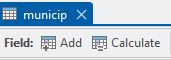
- At the top of the attribute table next to the word Field click Add button
- A new tab should appear in the attribute table called “Fields: Selected Municip” which allows you to edit the fields. Notice there is a new field at the bottom of the tab with a green box next to it
- Under the Field Name column, double click on the default label “Field” and type POPCHANGE in the bottom row with the green box on the left (the green box signifies that this is the field you are working on)
- In the same row (same field) under the Data Type column double click on the default and select Short from the drop-down menu (this means a short “integer” number will be used)
- When you are done, go to the Fields tab in the ribbon interface, on the top, and click on the save icon in the Changes group to save the new field.
- Click on the Municip selection tab in the attribute table and notice the new field at the end of the database (scroll to the end to see it).
- Click on the name of the new column and then click on the Calculate button located next to the word Add button at the top of the attribute table. This opens the CALCULATE FIELD dialogue box (you could have right click on the column name to reach the field calculator).
- In the Calculate Field dialog, the first part of the equation is already there: “POPCHANGE =” (under the Expression section). Population change is the difference between population in 1990 and 1980. You need to use the mouse to select the ‘Fields’ to create the following equation in the box below the = sign
“POPCHANGE =” !POP90! – !POP80!
Then, click OK.
The POPCHANGE column will update after a few seconds. Notice that there are fields with integer positive (population increase) and negative (population decrease) numbers.
- With the new population change attribute in your table, query the database of Municip selection to find municipalities that experienced little or no population decrease (we’ll use population loss value of less than 200; notice that since it’s a “loss” the actual value is -200!).
(Hint: Use the Select by Attribute function, and make sure you choose the correct layer in the first drop-down menu. Use POPCHANGE greater than or equal to -200 (notice the “-“ (minus) sign!). Remember: use the mouse as much as possible, only use the keyboard to type numbers).
Step #2 in cartographic model
- Leave this theme as is (with some municipalities selected) as we continue the exercise.
Question 6 – How many municipalities do you have left in your selection?
SPATIAL ANALYSIS
Queries based on spatial relations are of three basic kinds:
- Intersection (select features that are at least partially contained within other features)
- Containment (select features contained within other features)
- Proximity (select features within a certain distance of another feature)
Task 6: Intersection
The first type of query based on spatial relations is intersection. Here we will select features that are intersected (overlapped), to some degree, by a feature from another theme. The selected features are entire features, and not just the geographic location where the intersection actually occurs (as in raster analysis and other kinds of vector analysis).
Right now, we want to know which towns in our “remaining dataset” are intersected by large streams. This is done by using the Select By Location tool located in the Selection group under the Map tab in the ribbon interface. The Select By Location dialog box selects features from a theme that are in some spatial relationship with the features (or selected features) of another theme.
- The features to select are selected municipalities that
- Intersect
- Large streams (the features of another theme)
If we were interested in all streams, we could use the Select by Location right away; however, since we only want to consider large streams, first we need to select those streams using a single attribute query, making this a two-step process. In our database streams have different orders (1 – 5) that correspond to their size and volume.
- Display the Streams theme.
- Use the Select by Attributes tool to select streams with an order of 4 or 5 (these are the largest streams and rivers). By now, you should know how to do this. Use “greater than or equal to 4” to get the most accurate result easily (no quote signs). (Hint: you should have selected 111 features in Streams).
Step #3 cartographic model
- Now back to the municipalities (Selected Municip). To identify, out of the already selected towns, those that are intersected by the large streams, use the Select By Location option from the Selection group under the Map tab.
- Input Features: “Selected Municip”
- Relationship: “intersect”
- Selecting Features: “Streams”
- IMPORTANT: Selection Type “Select subset from the current selection”
- Click OK
Once the municipalities intersected by large streams are selected, you can now examine the attributes of those towns with the attribute table.
- Open the database table associated with the Selected Municip and select “Show selected records” (the right button on the lower part of the table window).
- Export the selected features in Selected Municip to a new theme as you did in step 26 with MUNICIP. Name it “Final_Municip”. Add it to your map (if it is not added automatically), and use this layer for the remainder of the exercise.
Step #4 cartographic model
Hint: you should end up with 7 municipalities. If not, something went wrong☹. Repeat the procedure until you get to this (Pay attention to instruction 36d, without this you’ll keep getting 17 municipalities). The rest of the exercise depends on this selection.
This is a good moment to save your map document and take a break, if you haven’t done so.
Task 7: Containment
Now, we have finished the task of choosing suitable towns. Next, we need to select the roads in these towns to continue towards our goal. To do this, we will use the Select by Location function again, but this time with a different spatial selection method, containment (or “something inside something else”).
- Display the ROADS theme.
- Choose SELECT BY LOCATION under the Selection group in the Map tab.
- Input Features: “Roads”
- Relationship: “Within”
- Selecting Features: “Final_Municip”
- Selection Type: “New Selection”
- Click OK.
Step #5 cartographic model
This operation selects those lines (roads) that fall within the features of Final_Municip (municipalities meeting our population criteria AND intersected by large streams). Roads within these towns appear blue.
Question 7 – How many roads are located in your selected towns? (Hint: >2000 and <3000)
Task 8: Proximity
The last of the queries based on spatial relationship is that of proximity. This form of selection allows us to select features that are within a given distance of another feature or set of features. In this case, we want to select roads (from our already selected set of roads) that are, at some point in their length, within 2000 feet of a public school.
- Display both ROADS (without clearing your previous selection) and PUBLIC.
- Use the Select by Attributes function to select features from PUBLIC theme of TYPE equal to ‘SCHOOL’ (make sure to select PUBLIC in the drop-down menu of the Select by Attributes dialog box).
Step #6 cartographic model
The second step of this proximity analysis is to select, out of the already selected roads, the ones that are within 2000 feet of the already selected schools. The steps for this procedure are as follow:
- Choose Select by Location in the Selection group under the Map tab.
- Choose as your Selection type “Select subset from the current selection” and set your Input Features as ROADS.
- PUBLIC is your Selecting Features.
- Your Relationship is “Within a distance”.
- Under Search Distance you will need to enter “2000” and “Feet” to set the correct distance
- Click OK.
Step #7 cartographic model
This operation selected those roads that are within 2000 feet of public schools. Look at the road layer (turn off all other layers, except Final_municip). There should be selected groups of roads/streets only within those few towns. Open the table of the roads layer to see your remaining suitable roads.
Question 8 – How many of the previously selected roads are within 2000 feet of public schools? (Hint: >800 and <900)
To avoid losing this multi-step selection, export the selection of roads as you have done before. Add the new layer to your map, and use this layer for the remainder of the exercise. Make sure that you only have roads inside the selected municipalities.
Once our query is complete, there are many ways to explore the resultant selected features/records. One way is to make a summary table that summarizes information from the attribute table. Now that you have found all of the roads to consider, you need to find out which town has the greatest length of suitable roads.
Task 9: Summarizing data
Using SUMMARY TABLE DEFINITION, we can create unique summary tables and save them in our PROJECT.
- Open the attribute table for your recently exported road data and notice the number of roads and the towns in which they’re located (in the MUN column).
- In the attribute table right click on the column heading for MUN and select SUMMARIZE. This will tell the SUMMARY TABLE DEFINITION function to make summaries based on unique objects in this column, i.e. towns.
- The dialog allows you to add several attributes to be summarized as well as the method of summary. In this case, you want to summarize length.
- Under “Statistics Field(s)” click on the drop-down arrow in the first white box (under Field) and select Shape_length (at the end).
- In the second white box (under Statistic Type) click the drop-down arrow and select “Sum”. This will add up the lengths of all roads in each town.
- Do not change the case field to summarize (should be MUN).
- Specify the location for the output table (it should be inside a GeoDB in in your working folder), name it with a meaningful name (like “road_town_summary”) (NOTE: Don’t use spaces, use underscore instead for the name) and
- Click OK.
Step #8 cartographic model
- The table will be placed at the bottom of the CP. Right click it and select OPEN.
The result is a small table that gives you the answer you need.
Question 9 – Which town should you visit? (I.e. the one with the longest length of roads) (Hint: right click on the Sum_Shape_Length column and choose “Sort Descending” to get the biggest length at the top of the table.)
Note: the summarized field, Shape_Length is an intrinsic field of the theme. It’s automatically calculated every time that the lines are modified. Its units are given in the layer’s coordinate system, in this case “Feet”. We’ll learn later how to get that info.
Notice that you can recall the table just created at any time from your map’s Contents Panel window where it is saved. In addition, you can add it to a new map as you add any data.
Before you save your project and begin part two of the exercise, find the town you would visit in the map. Then prepare a correct map showing: All the municipalities with the same color, the final municipality you chose (labeled and in a different color), your final selection of roads (only in the last set of selected towns), and insert all map components you know (title, author,legend, north arrow, and scale bar).
Export the map to PDF format (yourename_ex4_part1.pdf) and upload to Moodle.
Question 10 – Upload the map of part 1 to Moodle.
Now that you have completed part 1, this is a moment for you to study once again, and carefully, the cartographic model (flow chart) for part 1. Notice the data sources (primary and secondary) and sequence of steps/operations necessary to get to the result. This is a good planning tool for all GIS projects. Make sure you understand it and can follow it. You’ll be asked to make them later.
Part 2: Case Study – Multi-Criteria Evaluation (MCE)
The procedures used in the previous portion of the exercise were organized into a multi-criteria evaluation (MCE) problem where the objective was to find locations, or features, that meet several criteria. In this section, the problem is, once again, to combine several criteria that originate from different themes using a combination of queries by attribute and spatial queries.
You can think of the previous MCE problem in two stages. By doing single and multi-attribute queries, within the attribute table of each theme, we selected the records that met our criteria. This is a way of “standardizing” the data, i.e., making dissimilar data into similar (selected and unselected or “good” and “not good”):
- You used a single attribute query to select large streams from the theme STREAMS.
- A multi-attribute query was used to select municipalities with low population and low population loss from the theme MUNICIP.
After selecting (standardizing) each criterion the next step was to use them for a series of queries to be performed on the roads database. To find the best roads on which to live, we repeatedly queried the roads database based on the spatial relationships of containment (roads within low-density municipalities) and proximity (roads near schools). With each query we produced a smaller and smaller set of roads that are suitable given our criteria. The final result was only those roads that are suitable given all criteria.
In Part 1, you learned this process with step-by-step guidance. Now, you are ready to test your skills! In Part 2, you will complete a case study with less detailed instructions. Remember you can always refer to instructions in Part 1 AND to the cartographic model for Part 2 if you need assistance.
For this case study, your goal is to pick a Massachusetts county to live in. You have three criteria:
- you want your county to have a bicycle trail that is under construction (your profession is construction and your passion is cycling),
- you want to live near the MBTA railroad for easy access to Boston and its suburbs,
- And you want your county to have a junior college so your kids can pursue their studies close to home.
To accomplish your goal, you will repeatedly query the Counties theme based on the spatial relationships of Counties to other themes—bicycle trails, railroads, and colleges. You will use the Select by Attribute function to “standardize” the data in each of these layers prior to using them to query the Counties database—for example, you don’t want to query the Counties theme with all colleges, just junior colleges. In sum, you will be performing a multi-criteria evaluation, just as described previously.
STUDY CAREFULLY THE CARTOGRAPHIC MODEL OF PART 2 BEFORE STARTING.
- To begin, open a new ArcGIS Pro map (ex4_part2) using X:\e4 for location (don’t create a new folder). Then add the following themes inside the MAData.gdb geodatabase to the data view:
- COUNTIES
- Biketrails
- Railroads
- Colleges
Throughout this process, export the data to a new layer (to save your selections) as often as you want.
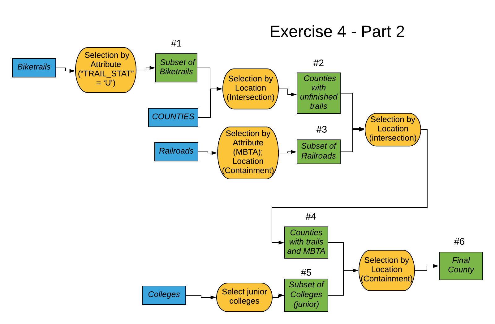
- Using the Select by Attributes function, select from the Biketrails theme, trails with a status (“TRAIL_STAT”) of underway (‘U’). (Hint: you should now have 22 bicycle trails selected. Check in the attribute table).
Step #1 of part 2 cartographic model
- Using the Select by Location function, select features from COUNTIES intersected by the selected trails. Check each setting in the dialog box to ensure that you are selecting the right set. (Hint: you should have selected 6 counties).
Step #2 of part 2 cartographic model
Question 11—Essex County is in the selected set. True – False
Continue to query the selected counties that contain the required type of trains.
- In the Railroads theme, you want only PASS_OP = MBTA (Passenger Operation; MBTA is the commuter system for Boston and surrounding communities). (Hint: you should have selected 817 railroad features).
Step #3 of part 2 cartographic model
- Now select counties with MBTA passenger-operated railroads. NOTE: you will need to be careful to select from the Select subset from the current selection in COUNTIES to preserve your previous selection from the bicycle trails (if you didn’t export the selection as a layer).
Step #4 of part 2 cartographic model
Question 12 – How many counties, intersected by the selected railroad features, remain as possible living locations? (Hint: less than 4)
- Continue to query COUNTIES: for Colleges, select only those with “junior college” in the description (“DESCRIPTN”). For this, sort the attribute table by “DESCRIPTN” in ascending or descending order, find junior colleges (there are 5), and manually selecting them by clicking the buttons on the left of the rows while holding the SHIFT key. For few items, this type of selection is easier than using the Select By Attributes function! (But you may do a selection by attribute, if preferred).
Step #5 of part 2 cartographic model
When you have selected the junior colleges, query the COUNTIES theme one more time.
Step #6 of part 2 cartographic model
Congratulations! You have found the perfect county for you to move in.
Question 13 – What county did you choose?
Featured image on top of page from Terrible Maps