Geog 210 – Exercise 3 – thematic mapping

Thematic Mapping in ArcGIS
Contents
- Part 1: Tutorial – Studying the Immigration and Unemployment Situation
- Objective: In this part of the exercise, you will learn more about how to produce a map (layout) in ArcGIS Pro through analyzing immigration and unemployment data.
- Part 2: Dr. John Snow and the cholera epidemic of London
- Objective: To analyze the spatial distribution of points and do basic table statistics.
- Part 3: Case Study – World Demographics
- Objective: Now you will apply your new mapping skills to analyze world demographic data
Part 1: Tutorial: Studying the Immigration and Unemployment Situation
One common argument against immigration hinges on its supposed impact on employment. But, does increased immigration actually bring greater unemployment? Through this tutorial, you will answer this question, and learn how to make maps in ArcGIS Pro. As background for this topic, read the article “What Immigration Means for U.S. Employment and Wages” by Greenstone & Looney.
Data for this project comes from “Parker, Robert Nash, and Emily K. Asencio. 2008. GIS and spatial analysis for the social sciences: coding, mapping and modeling”. You will be in charge of preparing the maps as you read excerpts of the study. Text in italics and indented is adapted from the text, text in regular font or left aligned shows your instructions.
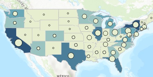
First, you will make a map of immigration and unemployment levels in the United States in 1994.
Task 1 – Preliminary tasks and adding data
- Copy the corresponding data folder (\ex3) into your X: drive (in future exercises, you will do this without a specific instruction).
- Start ArcGIS Pro and create a new project in ArcGIS Pro.
- Name it “immigration” or “Part 1”
- Save it in X:\ex3 (you have to navigate to your X drive under “This PC”: click once on the left panel of the “New Project Location” then select folder “ex3” on the right – don’t double click it- and choose OK)
- Uncheck to create a new folder for this project
- In the Map tab, click on the button for “Add Data” and add two copies of the theme US_Immigration (found in the Geodatabase called Exercise3.gdb inside folder \ex3) to the map.
- In the bottom copy, represent the field “unemp94” (it is a numerical field) using graduated colors, mono-color scheme, 5 classes. Rename the legend to “Unemployment 1994” (Get the Symbology panel by right clicking on theme name in the Content Panel. See Exercise 2 – Part 2 if needed).
- For the top theme, represent the field “imm94” using graduated SYMBOLS (not colors! Symbols!)
NOTE: Make sure the backgrounds (states) of the circles are transparent (it should be like that by default), i.e. the states don’t show a solid color. You should see the color of the states of the previous layer. Ignore the following instructions a-e if your symbols backgrounds are transparent and you can see different-sized circles on top of the previous layer.
- If you don’t have transparent background for your symbols (circles) click on the background icon in the symbology pane
- On top of the new pane (Format Polygon Symbol – Background) click on Properties
- Make sure the color for “Color” is set to “No color” (you can leave the default for “Outline color” OR also make it “No color”)
- Click Apply at the bottom
- You should have only floating circles (turn off the other theme to make sure) and the background color should be the “Unemp94” theme.
- Rename legend to “Immigration 1994”.
- On both themes in the CP, go to the Symbology pane and use the Method drop down bar to try Natural Breaks, Quantile, and Equal Intervals.
Which method do you think shows the unemployment data best? What about for the immigration data? Once you choose one use this classification method for the rest of the layers in this part in the exercise.
Task 2 – Preparing Layout (map printout)
- Go to the Insert tab of the ribbon and in the Project group click New Layout and select a Landscape Letter size paper (it could be portrait) (this will eventually show you the map in a page as if printed).
You will notice that a new blank window labeled “Layout” has been created next to your Map window in the center of your screen. You should also notice that a Layout tab has been added to your ribbon interface and that some of the tools in the other tabs have changed (pay special attention to the changes in the Insert tab as it contains most of the tools that you will be using to create the layout).
The first thing we want to do is add our map to the Layout.

- Click on the Insert tab in the ribbon interface and, in the Map Frames group, click on the drop-down arrow of the Map Frame button.
- Choose the image with colors and scale value (this is your map with the data that you added above). Do not choose Default Extent.
- Notice that the cursor changed shape: Draw a square in the blank page that takes about ¾ of the page. The map frame with your data should now be added to the layout. Notice that the corresponding themes have been added to the CP.

You can zoom in closer to your layout using the mouse wheel and pan around your layout by selecting the Navigate tool (located in the Navigate group of the Layout tab in the ribbon interface) and clicking and dragging on the layout with the mouse.

You can also change the size position of the map frame (as well as other map elements you will add later) in the layout by using the Select tool, which is located in the Elements group of the Layout tab. With the Select tool turned on, click and drag the map frame to move it or resize the map frame by clicking and dragging the sides of the frame. Try it!

However, these Navigate and Elements tools do not change the map itself. The map may look a little small when added to the layout or may be out of view slightly. To fix this, go to the Map group of the Layout tab in the ribbon interface and click the Activate button to activate the map frame and interact with the map.
Doing this allows you to pan around the map itself and change its position by left clicking and dragging the map. Try this until the map is positioned in the center of the frame.
You can also make the map bigger (zoom in), smaller (zoom out), or show the full extent of the map by using the tools in the navigate group of the map tab. Try this. You want to make the map as large as possible while also keeping all of the map in the view frame.

- Once the map is centered and zoomed in correctly, you should deactivate the map frame by clicking on the Layout tab in the ribbon interface and go to the Map group and select the Close Activation button to return to the regular layout.
Next, you want to add a title to your layout.
- Under the Insert tab go to the Graphics and Text group and click on the Rectangle Text tool (A).
- On the layout, above your map frame draw a rectangle (this is where you will add your title).
- Notice that in addition to your regular data layers a new Text layer has been added to the CP. In the CP, right click on the Text layer and select Properties (all the way to the bottom). A Format Text panel should appear on the right side of your screen.
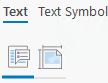
- The Text panel has a Text section and a Text Symbol section. Similar to the Symbology panel, towards the top of the Element panel under the Text section there are several icons with various functions. Click on the Options tab icon and find the white box under the word “Text” (you might need to click the arrow next to “Text”).
- In this white box type: “Figure 1. Immigration and unemployment in the United States, 1994” (no quotes); hit Enter and add your name in the second line (Map made by “Your Name”).
- Under the Text Symbol section, click on the word “Appearance” and change the size to 22 and hit apply at the bottom of the panel to see the title.
- Finally, adjust the size/position of the title to make it look good using the Select tool mentioned above (you might need to move the map frame or resize the rectangle by grabbing the corners and changing the size/shape).
Finally, you want to add some map elements like a Legend, North Arrow, and Scale Bar.
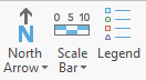
- Under the Insert tab on the ribbon interface go to the Map Surrounds group and click on the Legend tool (or the North Arrow, or the Scale Bar) .
- Draw a box on your layout to insert the legend for your map and use the Select tool to move it and resize it until it looks good.
- Repeat for the other two map components. For the scale bar, add a long horizontal rectangle.
- After adding the component, double click on it to get a property panel on the right.
- Make sure to get the properties of the scale bar and select the units in Miles.

If you want to change the orientation of the map (Landscape or Portrait): go to the Page Setup group in the Layout tab of the ribbon interface. In this group, click the down arrow under the Orientation tool and select Landscape. Rearrange the map frame and its components (title and legend) on the layout.
Take a minute to look at your map: Does it look good? Does it show the point that you want to make? Are the chosen colors adequate (not too outrageous)? Does the map have an adequate scale/size? Does the legend or title show correctly? No overlapping lines? Are you using the space effectively? Etc.
Make sure you arrange all the map elements well, with each element large enough to be readable. As a rule of thumb, scale bars are usually near the bottom, north arrows in some “upper” position.
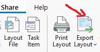
- When satisfied with how it looks, in the Share Tab in the ribbon click on Export Layout in the Output Group. This will cause an Export panel to appear where you can save your map in the X:\ex3 folder as a PDF file (Figure1_yourname.pdf). Make sure to click the Export button at the bottom of the panel to complete the export of your map.
NOTE: you have to choose File Type: PDF (*.pdf), it’s not enough to just type the extension at the end of the filename.
NOTE: Your map will be graded based on: 1- completeness (all required components are included); 2- content (the right data being shown); and 3- appearance (scale/size, page positioning, colors, labels, etc.).
You could select a graphic format, like PNG, if you plan to insert the map in a document like Word or PowerPoint, but in this case, we’re making standalone maps, so we use PDF. Always make sure that the layout you export (PDF or graphics) looks good. Go to the folder where you saved it and open it to make sure it is fine.
- Finally, in the CP rename Layout1 to Figure1.
- This is a good moment to save your map project (ex3_part1). Click the Save button on the very top toolbar (above the ribbon)
Question 1. Upload Figure 1 to Moodle.
Now, read carefully the following paragraph from Parker & Asencio (2008).
(Parker, R. N., & Asencio, E. K. (2008). GIS and spatial analysis for the social sciences. New York: Routledge)
As documented in the map’s legend, the graduated shades of light to dark indicate the unemployment level, and the graduated size of the dots (from small to large) indicates the immigration level. The map shows that for 1994 states such as California, Texas, and New York had high levels of both immigration and unemployment. Based upon this map alone, one might conclude that immigration and unemployment are correlated. However, if we look at the next map in Figure 2, showing a GIS of the immigration and unemployment in the United States for the year 2004, a different picture is revealed.
Did your map reflect what the text said? Yes? No? Then let us go on to create Figure 2:
- Return to the Map window (the little tabs on top of the central panel).
- Turn off the two 1994 themes.
- Add, to your map, again, two copies of US_Immigration theme (you can do copy/paste on the Contents pane, right click one of the previous layer’s name and choose Copy, then right click on “Map” in the CP and choose Paste).
- Repeat the previous instructions (steps 5-7) using the fields “unemp04” and “imm04”. IMPORTANT: Use the fields “04” for the data of year 2004.
- Use a different color scheme from figure 1
- Rename the legends accordingly (year 2004). Also, remember to remove the background for the graduated symbols.
- Create a new Layout and add the title “Figure 2. Immigration and unemployment in the United States, 2004” AND Your Name, as shown before.
- Make sure you add the Legend, North Arrow, and Scale to the layout (if you turn off the two themes from 1994 in the CP, they won’t show up in the legend).
- Make sure you arrange all the map elements well, with each element large enough to be readable. When satisfied with how your map looks, export (and save) your map as “Figure2_yourname” in the X:\ex3 folder as PDF (Figure 2_yourname.pdf). Then save the map project.
Question 2. Upload Figure 2 to Moodle.
Read carefully the following paragraphs Parker & Asencio (2008) and compare them with your maps. The narrative should describe the maps that you just made. You might want to compare the two maps that you have prepared.
The 2004 map shows unemployment to be high in states with high levels of immigration such as California, Texas, and New York as did the 1994 map. However, it also shows that states in which unemployment increased between 1994 and 2004 such as Nevada and Utah did not experience such an increase in immigration levels. Further, the maps show that the immigration level for states such as Washington, Oregon, Illinois, and Wisconsin declined between 1994 and 2004 despite a steady level of unemployment between these years. These findings indicate that the correlation between immigration and unemployment shown in these maps may be due to a spurious variable.
NOTE: you might need to use the inquire cursor to see these trends in these latter states
There are many potential sources of such a relationship between the unemployment rate and immigration. It is possible that the cause of the rise in the unemployment is entirely unrelated to the immigration. For example, massive layoff occurrences throughout the United States would cause an increase in unemployment, but has nothing to do with the number of legal and illegal immigrants in the country.
Data regarding massive layoff events (layoffs affecting 50 or more employees) in the United States for 1994 and 2004 were obtained from the Bureau of Labor Statistics to examine the relationships between unemployment, immigration, and the massive layoff events. The data regarding layoffs were included in the GIS to create the map of the United States in 1994 shown in Figure 3.
NOTE: You don’t need to upload the next two figures, 3 & 4 (steps 22-30) but you have to do them in order to practice your layout making skills. These two figures will help you to answer question 3.
To create Figure 3 (immigration, unemployment, and layoffs in the United States in 1994):
- Add two more copies of US_Immigration theme.
- Repeat the previous instructions using the fields “layoff94” and “layoff04” (Graduated symbols for both variables; transparent backgrounds). Use a different Symbol from the default circle (maybe squares) with a contrasting color.
- Rename the legends accordingly and arrange the order of the themes in the table of contents to show all 3 themes the best way possible (all 1994 together, all 2004 together).
- Make sure to keep all 2004 themes OFF when preparing figure 3.
- Add the title “Figure 3. Immigration, unemployment, and layoffs in the United States, 1994” and your name.
- Make sure you add only the correct legends to the layout.
- Add a north arrow and a scale bar.
- When satisfied with how it looks, save your map as “Figure 3.pdf” in the working folder.
Again, read the following from Parker & Asencio (2008), making sure that your map shows what is described here.
This 1994 map (figure 3) shows all of the states with the lowest unemployment also have the lowest number of massive layoffs, indicating a potential correlation between these two variables. States with larger populations such as California and Texas have higher levels of all three variables. States such as these that have more people tend to have more businesses, and therefore more jobs available that may attract immigrants. Because these states tend to support more and larger businesses than smaller states, they may be more prone to massive layoffs than smaller states. The same map for 2004 appears in Figure 4.
- Prepare the layout for figure 4 with the 2004 immigration, unemployment, and layoff data. Use the right title and legend. Save your map as “Figure 4.pdf”. Then save the map document.
Study the following paragraph from Parker & Asencio (2008) that relates to figures 3 & 4. Make sure that your maps show what it is described here.
The 2004 map shows an increase in massive layoffs in Nevada and Utah from that in 1994. Recall that immigration levels did not change in these states between 1994 and 2004, but unemployment increased during this period. Based upon the addition of the massive layoff data, it appears that the unemployment rise is more likely correlated with the massive layoff events than with immigration. However, there are other states such as Georgia in which the number of massive layoffs increased between 1994 and 2004, but the unemployment rate did not change. This indicates that there may be still other variables outside of the current model that accounts for the spurious relationship between unemployment and immigration.
Read the article “What Immigration Means for U.S. Employment and Wages” by Greenstone & Looney, if you haven’t done so already, before answering the following question:
Question 3 (Not optional). Based on your GIS research and readings (assume that they’re still current), would you support or dispute the following statement? “Immigrants in the U.S. are taking jobs away from Americans and lowering wages”. (No wrong answer; but do explain it using the evidence provided in your GIS project)
Part 2: Dr. John Snow and the cholera epidemic of London
In class we introduced you to the case of the cholera epidemic in London, mid 1800’s. Read the text provided in Moodle for a more complete introduction. In this part of the exercise, you will do a basic spatial analysis of point data by studying the distribution of cholera death cases and the water pumps in this sector of London.
NOTE: The dataset used in this part was obtained from Robin Wilson’s blog. More information about this interesting case of GIS and epidemiology history can be read in the Wikipedia article Dr. John Snow and the Cholera Outbreak
Task 1: Getting started and adding data
NOTE: Using the knowledge acquired in Part 1 you should be able to work more independently in this section; therefore instructions will be more limited.

- Create a blank map in ArcGIS Pro. If ArcGIS Pro is open with previous map click on the icon that looks like a blue box with a sun on the very top left of the window.
- Create a blank map in ArcGIS Pro with an appropriate name and location.
- Remove, or turn off, World Hillshade, but leave World Topographic Map
- Add the image called SnowMap.tif in the \ex3 folder to the CP
Take a minute to explore the image. Zoom in and move around so you can see the way Dr. Snow annotated the map. At each address, he placed a mark for each death (this map is a little fuzzy; check the original in Wikipedia for a better quality image). He also indicated the locations of water pumps. Notice how the map is not perfectly square, but it has some distortion, visible along the edges. This is because the original map was scanned, then “georeferenced” to give it real world coordinates.
- Turn off and on the two images to confirm that both are correctly aligned. Notice that some streets have changed.
- Turn off World Topographic Map and leave SnowMap on. Now add the Water_Pumps and Cholera_Deaths themes from inside Snow_Cholera_Data geodatabase. Change the default icons into something easier to see and put the water pumps on top of the cholera deaths in the CP.
Task 2: Exploring the data
Again, take a minute to explore the data. Zoom in so you can see that there is one point of cholera death for each address. Also check the points of the water pumps, make sure they are correctly placed.
- Using the Explore tool (Map tab in ribbon) click on one of the death points. Notice that there is an attribute called Count, can you guess what that is?
- Represent the theme Cholera_Deaths using graduated symbols with the Count column. Accept the default classification.
- Open the attribute table of Cholera_Deaths and sort the Count column (right click on the theme in the CP and choose Attribute Table, or click once in the theme in the CP and then the tab Feature Layer\Data and push the Attribute Table button).
Question 4. How many addresses are listed in the table (Hint: Notice the number at bottom of the table)
Question 5. What is the largest number of deaths that happened at one address?
- Right click the heading of the column Count and choose Statistics. Study the result in the new panel. It contains statistical information about numerical variables. The “Count” value should be the same as your answer for question 4 and the Max value is your question 5.
Question 6. What is the total (Sum) number of cholera cases in the dataset?
- Close the Attribute Table and Stats panels and right click on Water_Pumps, in the CP, and choose “Zoom to Layer” to see them all in the Map panel. Make sure that you can see clearly all the points, including the water pumps. There is clearly one pump in the center of most of the death cases. Use the Explore tool to learn the name of that pump.
Question 7. What is the name of the water pump in the center of most casualties?
- READ THIS WHOLE INSTRUCTION FIRST, BEFORE DOING THE FOLLOWING

- Click on the Select tool located in the Selection group of the Map tab and select the water pump identified above. It should turn blue.
- Then, click on the Select by Location tool (also located in the Selection group of the Map tab).
- Once this tool opens, under Input Features click on the drop-down arrow and select Cholera_Deaths,
- under Relationship click on the drop down-arrow and choose Within a distance,
- under Selecting Features click on the drop-down arrow and choose Water_Pumps,
- and under Search Distance type in 100 and change the units to Meters using the drop-down arrow.
- Click OK and notice that all of the death cases within a distance of 100 m of this dirty pump must now look bright light blue (it means that they are selected).
- Open the attribute table of the Cholera_Deaths theme, notice some lines/addresses selected in blue. Open the statistics of the Count variable. This time the stats are calculated also on the selected features.
Question 8. How many deaths occurred within 100 m of this water pump? (HINT: notice that there are two columns of results in the Statistics pane: Dataset & Selection; pick accordingly)
Of course, this assumes linear distances from the water pump. People will travel through the streets. Using an advanced GIS technique called Network Analysis, you can determine the area around the pump that represents a particular walking or time distance.
You could repeat this analysis around the other pumps to verify if there are more or less casualties within their corresponding areas.

- Clear the previously selected features by clicking on the icon to the far right in the Selection group (white square)
Task 3: Preparing layout
- Prepare a good layout containing Snow’s map as background, the death cases as graduated symbols and the pumps clearly visible. Make sure to zoom in to the important area (cholera cases), no need to include the whole city! Insert title (with your name), legend, scale bar, north arrow, and use the tools in the Graphics and Text group under the Insert tab of the ribbon interface to annotate the map indicating the “guilty” water pump and label it with its name. Save the layout as PDF (Snow_map_yourname.pdf, part2_map_yourname.pdf, or something suitable). Refer to the grading criteria given previously.
Question 9. Upload map to Moodle.
Part 3: Case Study: World Demographics
(Adapted in part from Exploring Environmental Science with GIS by Stewart et al. 2005)
One of the most exciting aspects of working with GIS is the ability to make your own maps by combining multiple layers and comparing variables among places. Now that you have learned how to do this, and practiced your map making skills, you will create a map of global demographic factors and become more familiar with the functions of ArcGIS you have learned so far.
Task 1: Getting started and adding data
- Create a blank map in ArcGIS Pro. Turn off the two background layers (World Topographic Map and World Hillshade) and add the World_Demographics theme inside Exercise3.gdb. Use the Explore tool to answer the following questions.
Question 10. What is the population of the United States in 1980 (POP1980) according to this dataset? (Count the # of digits carefully, and don’t use commas in Moodle)
Task 2: Mapping attributes
All the attributes of this dataset, except for country names, FIPS, and continents are numerical, but right now, the map is just showing one common color for all countries, i.e. it is showing only locations.
- Open the attribute table and familiarize yourself with its contents.
Question 11. How many individual features (countries/territories) are represented in this map? (Hint: look at bottom of table)
Question 12. Which country had the highest population in 1950?
- Close the table and represent the population in 2020 with graduated colors (5 classes, natural breaks).
Question 13. Of the following list of countries choose the two that show the highest population values (Hint: the highest two categories might show with very similar colors. Click on the color symbol for the highest category and change the color to a contrasting one)
Australia – United States – India – Canada – China –Brazil – Spain
A population map sometimes is not very informative. There are two problems with it:
First, it shows total values, the number of people per country. Since large countries often have large populations, mapping total values by color classes can be confusing: for example, how do you know whether a population is dense or simply expansive? You should be cautious mapping total values using area-shading (“choropleth”) mapping. Instead, map the rates, such as population per square mile or births per 1,000 people, some unit of “density”.
A second reason for the lack of information in your population map is that the data range is not well represented. You cannot see a good deal of the distribution because one or two countries have such extremely high values that the rest of the world falls in the bottom one or two classes.
- To correct the problem of the total values, try mapping population density in 2020 (DEN2020), and play around with the classification until you are satisfied. Is the value pattern of people distribution now a little different?
Question 14. Using a Quantile classification with 5 classes, is there any country in the Western hemisphere (American continent & islands) with a population density in 2020 that falls in the top category? Yes – No
Let’s try a different attribute. This time use BRTHP000, which is the number of births per 1,000 people, using graduated colors. This variable should offer a more visually interesting map; with greater variation among the countries.
Question 15. Which continent has the highest number of countries with high birthrates?
Question 16. What is the birthrate of Dominican Republic (South east of Florida)? ___ births/1000 people
Question 17. What is the birthrate of Haiti (next to previous)? ____ births/1000 people
- Now map death rates per 1000 people (DETHP000) using graduated colors.
Question 18. Which continent has the highest number of countries with high death rates?
Question 19. Which, out of all the countries in this dataset, is the one with the highest death rate?
Question 20. What is the death rate of Dominican Republic? _____ deaths/1000 people
Question 21. What is the death rate of Haiti? ____ deaths/1000 people
Question 22. What could account for the differences in birth and death rates between the Dominican Republic and Haiti? Notice that both countries share the same island of Hispaniola. Do a brief research about these countries to substantiate your answer.
Task 3: Make and explain your own map
The World_Demographics theme has many attributes available. Try mapping one or two additional attributes. For each, pause to look at your map, both globally, and by zooming in, regionally. Can you identify countries with high/low values of your selected attributes? Can you propose some explanations for those highs and lows?
Descriptions for all field are shown in the appendix at the end.
Your final task in this exercise is to create a map(s) of your choice of variables, and to analyze the pattern(s) this map(s) shows. Choose at least two variables to represent (look for interesting trends or patterns to explain in your analysis) and create a full map layout (it may contain one or more maps) using the skills you have learned. It does not need to cover the whole world. You may select a region or continent to focus on.
Export your map as PNG (this does not degrade the image like JPEG, but it is still easy to insert into another document). Create a Microsoft Word (or Google Docs) and insert your map. Below your map, type one or two paragraph(s) explaining what variable(s) you mapped, identifying a country or region with especially high value and a country or region with especially low values. Then, discuss what reasons or causes may lay behind the patterns you observe. Save the document with your name.
Question 23 – Submit your document (PDF or MSWord.NOT Pages; I have to read it) with the map(s) and discussion. Don’t forget required map components (also include your name in the filename and inside the document)
Appendix to Part 3: Data Dictionary
Many GIS programs require short attribute names. As a result, attribute names (field names) are often cryptic. These are the attributes in World_Demographics. All data not dated are most recently available records or estimates, as of 2003. Data source: US Census IDB
| Item Name | Definition |
| FIPS_CNTRY | Country identification code |
| CNTRY_NAME | Name of country |
| POP1950 | Population 1950 |
| POP1960 | Population 1960 |
| POP1970 | Population 1970 |
| POP1980 | Population 1980 |
| POP1990 | Population 1990 |
| POP2000 | Population 2000 |
| POP2010 | Population 2010 (projected, as of 2003) |
| POP2020 | Population 2020 (projected, as of 2003) |
| BRTHPOOO | Births per 1,000 people |
| DETHPOOO | Deaths per 1,000 people |
| MIGRPOOO | Migrants per 1,000 people |
| NETINPCT | Net increase, percent per year, including births, deaths, immigration, and emigration |
| BIRTHS | Number of births per year |
| DEATHS | Number of deaths per year |
| NUMMIGR | Number of migrants per year |
| NATINCRS | Natural increase (births, deaths alone) |
| POPCHANG | Population change, in number of people |
| FERTPWOM | Fertility per adult woman |
| IMRBOTH | Infant mortality rate, male and female |
| IMRMALE | Infant mortality rate, male |
| IMRFEMALE | Infant mortality rate, female |
| LIEXBOTH | Life expectancy, male and female |
| LIEXMA | Life expectancy, male |
| LIEXFEM | Life expectancy, female |
| DEN1950 | Density, persons per square mile, 1950 |
| DEN1980 | Density, persons per square mile, 1980 |
| DEN2000 | Density, persons per square mile, 2000 |
| DEN2020 | Density, persons per square mile, 2020 |
| SQKM | Area, square km |
| SQMI | Area, square miles |
Featured image on top of page from Illustrated Guide to NonProfit GIS (link in Moodle)