Raster analysis
Contents
- Part 1: Terrain Analysis
- Objective: Perform interpolation to create a digital elevation map (DEM), calculation of slope/aspect, and reclassification of rasters to locate the best place for a solar farm.
- Part 2: Zonal Operations
- Objective: Perform zonal statistics.
- Part 3: Watershed analysis
- Objective: : To delineate the watersheds of the Dean and Roaring Brooks and the west branch of the Swift River, and calculate their respective areas
Part 1: Terrain analysis
In this part we want to find the best place for a solar farm. The selected site must be on a relatively flat area (slope 0-5 degrees of inclination) and where it gets the most solar radiation during the day (a south facing area). In addition, it must be a single parcel larger than 60 acres.
NOTE: Keep track of the procedures, you’ll have to make a cartographic model at the end.
Data: You don’t have direct access to a Digital Elevation Model (DEM) of your area of interest (AOI) but a good friend has provided you with an outline of the area, AOI (North of South Hadley) and a regular sampling of points with their elevation values (Elevation_Points).
First, we need to create a DEM from the point data through a process called Interpolation.
Interpolation predicts values for cells in a raster from a limited number of sample data points. It can be used to predict unknown values for any geographic point data, such as elevation, rainfall, chemical concentrations, and noise levels.
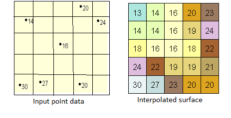
We’ll use a method called Inverse Distance Weighted or IDW:
This method assumes that the variable being mapped decreases in influence with distance from its sampled location. E.g., when interpolating a surface of consumer purchasing power for a retail site analysis, the purchasing power of a more distant location will have less influence because people are more likely to shop closer to home
Task 0 – Preliminary – Data source and activating Spatial Analyst extension
The dataset for this exercise is in the usual place (N:\Geog207\ex7) copy the whole \ex7 folder to your working folder and work there. This dataset is larger than previous and it might take some time to copy.
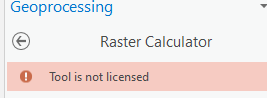
After copying the data you need to verify that ArcGIS Pro has the right permissions. It needs an extension called Spatial Analyst to work with raster. We have the extension installed but before using it we need to activate it. If it’s not activated, you’ll get an error message when using some raster tools.
After launching ArcGIS Pro, before creating a map or opening an existing map, click Settings, on the left, then Licensing … OR if you already loaded a map go to the Project tab (first tab on the left) Licensing. In the box “ArcGIS PRO extensions” verify that Spatial Analyst is licensed, If YES, you’re OK, keep working. If NOT, click the button “Configure your licensing options” below and check the checkbox next to Spatial Analyst. Click OK and continue working.
NOTE: Spatial Analyst is a very old software that ESRI hasn’t updated in a long time so it cannot work with blank spaces in the paths (folder names) or file names. Use “_” underscores if necessary. E.g. “X:\user\My folder\my data” will not work, use instead “X:\user\My_folder\my_data“
Task 1 – Creating DEM and calculating Slope and Aspect
- Create a new map project in a new working folder containing the required dataset.
- Add the vector file Elevation_Points located in Terrain.gdb to your map and open the attribute table; notice the column containing elevation data in meters.
- In the Analysis tab click the red Tools icon and in the Geoprocessing pane on the right, click on Toolboxes on top, then go to Spatial Analyst Tools > Interpolation > IDW
- Enter Elevation_Points as input
- Z value (this is the elevation value to be used in the DEM) should be set to the elevation field
- Output raster, save it as DEM_AOI (no empty space in name)
- Output cell size enter 30 (meters, don’t enter the units; units depend on the map units, meters)
- Leave all the other fields as they are and click Run.
Study the resulting raster. Verify its properties and make sure the cell size is 30 (R-click on the theme > Properties >Source > Raster Information)
Question 1. How many columns does this DEM have?
The raster will show in the map window with about nine discrete classes. Please note the color changes and the values in the legend carefully and study the terrain. Can you see which areas are lower in elevation? Where are the higher elevations?
Question 2. In general, in what direction is the elevation going up?
From North to South – South to North – East to West – West to East
Now we need to calculate the Slope. This is the inclination of the terrain, or rate of change in elevation by change in distance. You can express it as a percent change or in degrees of the angle θ (see figure).
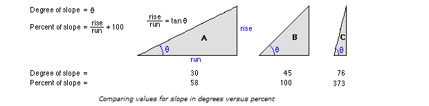
- % Slope = (a/b) x 100 where “a” is the change in elevation (Rise) and “b” is the change in distance (Run)
- Slope in degrees = Arctan (a/b) (Arctan is the inverse tangent function of the ratio a/b; remember that a/b is Tan θ)
- Notice that a 100% slope is a 45-degree angle, larger angle will give you a slope > 100%
Knowing the elevation of each cell and their size (in our case 30m) the software calculates all the slopes (in either percent, %, or degree, °) around each cell and outputs the steepest slope for the center cell. We’ll use slope in degrees.

- Go to the Analysis tab click on the red Tools icon
- In the Geoprocessing pane click on Toolboxes on top then go to Spatial Analyst Tools > Surface > Slope
- Enter DEM_AOI as input
- Enter Slope_degrees as output
- Output measurements as DEGREE
- Leave Z factor at 1 (the vertical, height, values are in meter, same as the XY coordinates) and Run.
Study the result. You should get values between almost flat (0 degrees) to around 17 degrees. If the software is showing you values up to ~90 degrees, go to the symbology pane of the layer and choose a Classify symbology with Natural Break 5 classes. The legend should now show you the minimum and maximum values.
Now we need to find the areas that are facing the sun. In the northern hemisphere, the sun is always on the southern side of the sky above us (remember that the sun shines perpendicular in tropical regions). We need to find areas where the slopes are facing south. This is the Aspect of the slope.
Using a compass as a guide, and knowing that a circle has 360 degrees around, we assume that north is 0º, east is 90º, south is 180º, and west is 270º (see figure).
- Go to the Analysis tab click on the red Tools icon
- In the Geoprocessing pane click on Toolboxes on top then go to Spatial Analyst Tools > Surface > Aspect
- For input use the DEM_AOI (NOT the slope raster)
- Save the output as Aspect_AOI.
Again, study the results: it should be very colorful. Notice the legend and copy the range of angles shown for South ________________ (copy these values). All aspects between those values are facing south and good for our solar panels. These directions should be represented light blue in the CP, similar to the graph above. Look at the map and try to see which areas have these colors. Compare it with the original DEM. Can you see the south facing areas in the DEM?
Notice also that there is a class for “flat” areas with a value of -1. Flat areas have no slope orientation.
Task 2 –Reclassification and overlay
Now we need to put those two themes (slope & aspect) together. However, even though they both have units of degrees, they represent different things. One represents degrees of inclination in the vertical direction; the other represents degrees of orientation from the north (in the horizontal direction). We are going to separate the “Good” areas, just as we did with vectors in Exercise 6 land suitability. This is called Standardization, i.e. taking layers that represent different things and making them compatible. We do this, in raster analysis, with a function called Reclassification.
Reclassification assigns new numbers to our raster cells according to our criteria. In the case of the slope we are going to reclassify all the values with a slope of 0-5º (i.e. flat) to have a value of “1”, all the other values will have a value of “0”. For the aspect, we’re going to assign a value of “1” to our south facing slopes, and “0” to the rest.
- Go to the Geoprocessing pane (Analysis tab Tools), click on Toolboxes on top, then go to Spatial Analyst Tools > Reclass > Reclassify
- Input: Slope_degrees (NOTE: use the SLOPE raster!)
- Reclass field: Value
- In the Reclassification table, make sure the first Start value shows the first class from the lowest value (0.008145, or just “0”) in the Start column
- Enter a value of 5 in the End column of the first line, leave the New Value for this first class as 1
- For the second class, enter 5 for start and 99 for End, change the New value to “0” (Any number higher than 17.32 will be good for the End field, 99 or 9999 is a “save” easy number)
- Leave the NoData as it is
- Left-click on the “extra” lines and press the delete key in the keyboard to remove them. Make sure there are only 3 rows: 0-5, 5-99, and NoData
- Output raster Good_slopes.
- Click Run.
You should get a binary (0/1) map. It’s important that you get a raster with only 0 and 1 value (this is called a Binary or Boolean raster). If you got values 1 and 2, you didn’t assign the classes correctly, do it again.
Study the output; everything with a value of 1 is Good (relatively flat).
Since this is a raster with integer values, it does contain an attribute table, open it and check its content.
Hint: Good_slopes should have 29971 pixels with value of 1.
Now try to open the attribute table of the DEM, or the slope, or the aspect raster. You can’t, do you know why?
- Now reclass the Aspect raster.
- Input: Aspect_AOI (NOT DEM)
- Reclass field: Value
- In the Reclassification table enter, in the first row, a value -1 to 157.5, change the New Value for this first class to 0
- For the second class, 157.5 to 202.5, change the New value to “1”
- For the third class, 202.5-360, change the New value to 0.
- Leave the NoData as it is and delete the extra rows. You should end up with 4 rows
- Output raster Good_aspects. Click Run.
Again, you should get a binary (0/1) map, if not, do it again.
Hint: Good_aspects should have 5130 pixels with value of 1.
With vector layers, we would now do an intersection to find the sites where the two good conditions coincide. In raster we use a trick from basic math: all numbers multiplied by 0 become 0. So we’ll just multiply our binary (0/1) maps and only in the places where cells with value 1 overlay another cell with value 1, there will be a 1 as a result. See the table below. That is why it was important to have only 0’s and 1’s in our “Good” maps.
| Good_Slopes | Good_aspects | Good_areas | ||
|---|---|---|---|---|
| 0 | x | 0 | = | 0 |
| 0 | x | 1 | = | 0 |
| 1 | x | 0 | = | 0 |
| 1 | x | 1 | = | 1 |
- Use the Raster Calculator (Geoprocessing pane Spatial Analyst Tools > Map Algebra > Raster Calculator) to multiply Good_slopes and Good_aspects and name the output Good_Areas.
- In the Raster Calculator pane double click on the 1st layer (e.g. Good_aspects) then double click on the * symbol then double click on the 2nd layer. You “build” the following equation “good_aspects” * “good_slope“
- Name output: Good_Areas
- Examine Good_Areas. Only the few pixels with value of 1 are suitable for our purpose.
Question 3. What’s the total area of “Good_areas” in acres?
Hint 1: Only pixels with value of 1 (suitable).
Hint 2: Check the properties of the final raster to find out the area of one pixel, and the units of the map (R-click on theme>Properties>Source>Raster Information)
Hint 3: Knowing the area of 1 pixel, the attribute table tells you the number of pixels, so calculate the total area. This area will be in map units square. Convert those units to acres.
Very small patches of land are not good enough for a solar farm, so the total area calculated is not very realistic. One final thing we need to do is to dis-aggregate all the separate patches (groups of touching pixels) with value 1 (equivalent, in the vector world, to converting a multipart polygon to single part). Then we can extract the ones larger than certain critical size (in our case, how many acres? ______)
- In the Geoprocessing pane launch Spatial Analyst Tools > Generalization > Region Group
- Input Good_Areas
- Output Regions_good_areas
- Number of neighbors FOUR (this decides which “touching” cells are counted as a group: FOUR – only cells touching up/down and left/right; EIGHT – same as before plus the diagonal cells)
- Leave the other options with the default values and click Run.
Display Regions_good_area using a symbology of Unique Values and study its attribute table. Notice the large number of new groups (regions or zones) created. They have all been assigned a new Value, but they still have the information of suitable/unsuitable (1/0) in the column LINK, and, of course, the Count column tells you how many pixels there are in each region, therefore you can calculate the area of each patch of land.
HINT: There should be 328 regions
Question 4. How many groups of cells (regions) are SUITABLE?
Hint: 1’s
Question 5. How many suitable parcels (regions) are larger than 60 acres?
Hint: you need to calculate how many cells are in 60 acres
In theory, we would also need to consider other factors like accessibility (distance to roads), environmental protection (buffers around water bodies), etc. but that’s a problem for another day.
Question 6. Make a correct cartographic model include your name in the model and in the file name, and upload to Canvas in PDF format.
Hint 1: It’s very simple.
Hint 2: End it with the creation of Regions_good_areas
- Save your map. It’ll be used in the next part.
Part 2: Zonal operations
Task 1 – Zonal statistics.
After you explored the suitability of the area to have solar panels, a dispute among the neighbors has erupted. They want to know how much of their land is suitable for solar panels and whether their homes are located in suitable areas.
To solve these problems, we’ll use a Zonal operator to evaluate Good_Areas using the neighbors’ parcels (polygons) and houses (points) as “zones”
- Open the map from the previous part and add the layers AOI and Houses to your map (If you just have a new blank map, bring also Good_Areas and DEM_AOI)
The houses theme contains the information of the owner, but the parcels shown in AOI don’t have owner’s name (check both layers’ tables). Therefore, we have to join these two.
- Do a spatial join (Intersection) on AOI (target feature) with the houses theme (join feature).
- Study the attribute table of AOI and make sure the names of the farmers are there.
- Go to Geoprocessing pane Spatial Analyst Tools > Zonal > Zonal Statistics as Table (read the help of the tool to learn what it is that you’re doing)
- Input raster or feature zone data (i.e. the file that defines the “zones”) – AOI
- Zone field – Name (aoi_AddSpatialJoin.Name)
- Input value raster (i.e. the raster to be evaluated) – Good_Areas
- Output table – ZonalStats_Parcels
- Statistics type – ALL
Study the output table. It shows a series of statistics for all the pixels from Good_Areas that fell within the limits of each parcel. Since the analyzed raster was a binary raster most of those columns don’t make sense, except SUM that shows you the sum of the values of all the pixels in the parcel. Since all the pixels only have values 0 and 1 their sum is the same as the total number of pixels with value 1. Notice that the column COUNT now includes both, pixels 0 & 1, it’s just a total pixel count.
Question 7. Which is the parcel (name) with the largest number of good pixels (with value 1)?
Question 8. What is the total number of acres in the parcel above?
Hint 1: NOT just good pixels.
Hint 2: don’t use the “AREA” column; the COUNT column tells you how many pixels there are, multiply these by the area of one pixel
Question 9. How many acres of good area are in this parcel? (Hint: <300)
Finally, let’s redo this zonal statistic using DEM_AOI as our Input value raster.
- Go to Geoprocessing pane Spatial Analyst Tools > Zonal > Zonal Statistics as Table
- Input raster or feature zone data (i.e. the file that defines the “zones” – AOI
- Zone field – Name (aoi_AddSpatialJoin.Name)
- Input value raster (i.e. the raster to be evaluated) – DEM_AOI
- Output table – ZonalStats_DEM
- Statistics type – ALL
Study the output table. Now, some of the calculated statistics do make sense. You can now see for each parcel the minimum and maximum elevations (range is max minus min), the average elevation, and the standard elevation. In this case the column SUM is the one that doesn’t make sense (can you tell why?).
Question 10. What is the average elevation for White parcel?
Question 11. What is the highest elevation found at Black parcel?
- Save and close the map
Part 3: Watershed analysis
Adapted from Spatialabs 2013
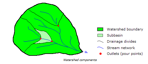
A watershed or drainage basin describes the area of land from which all surface waters (rain, melting snow or ice) converge at a single point. This point is the exit of the watershed and usually forms a stream or lake. Watersheds are important hydrologic and environmental units because all water within one watershed is connected. Thus, water pollution at one point in the watershed will affect the entire area downstream of that point and thus becomes an important issue in environmental restoration and protection. Since water always flows from the highest point to the lowest, watershed boundaries (drainage divides) are defined as the ridges separating flow.
The problem
The geology dept. at MHC has an ongoing study on the surface and subsurface hydrology in the town of Shutesbury, located just west of the Quabbin reservoir. In this town the US Geological Survey (USGS) has installed 3 river gauges that track the surface water flow at Dean and Roaring Brooks and in the west branch of the Swift River, a major source of water to the Quabbin. By determining the extent of the land area that contributes water to these streams, and eventually to the gauges, we can study different aspects of the hydrology of the area.
Objectives
To delineate the watersheds of the Dean and Roaring Brooks and the west branch of the Swift River, and calculate their respective areas.
Data description
The dataset in Watershed.gdb in your working folder is already clipped (see note below) to our Area of Interest (AOI):
- Digital Elevation Model (DEM_AOI) and the hill shaded version (use the hill shade, with 50% transparency, on top of the other layers for display purposes, it just looks cool!)
- Pour points (USGS Gauges), both vector (Gauges) and raster (pour_points_raster). The raster version is hard to see so the vector has been provided for visualization, the analysis will be done with the raster
- Streams (HYDRO25K_ARC_AOI)
NOTE: This part also uses the extension Spatial Analyst, if you haven’t done it you need to activate it as shown in Part 1 Task 0 (or if you moved to a different computer)
NOTE 2: To clip a raster you cannot use the usual Clip function. You use the function “Extract by Mask” under Spatial Analyst Tools>Extraction, but you don’t need to do it
Task 0 – Load the data in the Watershed geoDB and study it
Delineating watersheds
Delineating watersheds in GIS requires several steps including (detail instructions are shown below)
- Filling sinks in the elevation model
- Determining the direction of water flow through each grid cell
- Identifying stream channels, flow accumulation
- Determining the set of adjoining cells that contribute water to a particular pour point watershed.
This process requires several input datasets derived from the DEM that need to be created first. These are: filled sinks, flow direction, and water accumulation. And we also need the location of the gauges or pour points.
Task 1- Create a hydrologically correct DEM by filling any artificial holes (sinks) in the data.
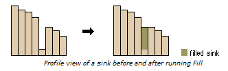
Sinks represent depressions (real or erroneous) in your data that impede water flow and therefore must be removed. The software fills the sinks by raising their elevations to equal neighboring cells so that water can continue to flow across them.
- Fill the sinks in the DEM
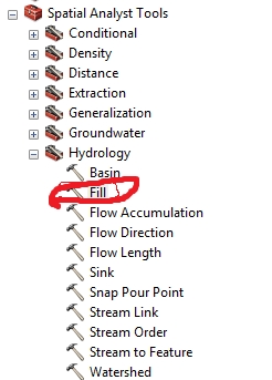
- Toolbox » Spatial Analyst Tools » Hydrology » Fill
- Input surface raster – DEM_AOI
- Output surface raster- filled_DEM
- Assign the same color scheme to both filled_DEM and DEM_AOI and compare them (there are several color schemes suitable for elevation).
Can you see any difference between the two DEM’s? Don’t worry, puny humans can’t tell the difference between these but the computer can 🙂
Task 2 – Determine which way water flows from cell to cell
- Determine flow direction for your filled DEM
- Spatial Analyst Tools > Hydrology > Flow Direction
- Input here is filled_DEM
- Output – flow_dir
Water always flows from high values (elevation) to low values. The flow direction layer looks strange but if you look at it carefully it will start to make sense.
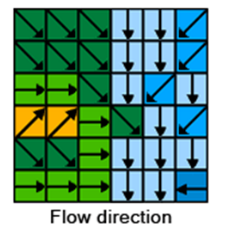
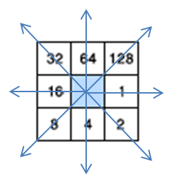
The legend will have numbers in from 1 to 128 according to the figure on the right. Cells with values of 1 are cells flowing to the East, south flowing cells have a value of 4, 16 to the west, and 64 to the north. You could change the legend values using the symbology pane to make better sense of the image. See figure below fora suggested legend.
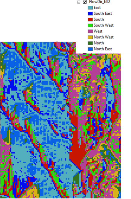
Look for areas of contrasting color changes and study the legend, you should be able to see where the flow of water changes from ‘East to West’ (i.e. west direction) to ‘West to East’ (east direction). See figure on the right for example and the figure below for a concept of water flow, remember the water will flow from higher to lower elevations.
Task 3 – Determine where water accumulates.
- To determine where water accumulates and creates channels, go to:
- Spatial Analyst Tools > Hydrology > Flow Accumulation
- Use flow_dir as input
- flow_acc as output.
- Invert the color scheme to show a water accumulation (streams) darker on a white background: Double click the color rectangle (legend) of flow_acc to go to the Symbology pane and tick Invert color box.
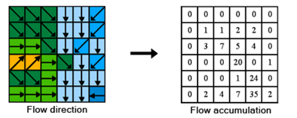
You can just barely make out some of the stream channels. Every cell has a numerical value equal to the number of cells that “provide” water to it (see illustrations)
This raster layer could serve as a proxy for a hydrology layer (streams) if we don’t have this as it shows areas where water accumulates over the terrain. The value of one cell reflects the number of cells, above it, that contribute water to that particular cell. You might need to reclassify the raster to “determine” what can be considered a stream and what not (a 0/1 raster). Also, you might have to vectorize the result.
Using this raster, you can also do some extra hydrological analysis like stream orders.
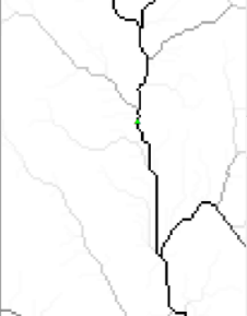
- Turn on (and off) the Hydro25K_Arc_AOI layer and notice the similarities and differences.
- Also, click on different water accumulation pixels in the raster layer (turn off ALL layers except Flow Accumulation). Notice how the pixel values change in different parts of the streams. Darker pixels should have larger values than lighter ones. These numbers represent the numbers of cells that contributed water to that particular pixel where you clicked.
Task 4 – Determine watersheds
You are finally ready to delineate watersheds.
- Spatial Analyst Tools > Hydrology > Watershed
- flow_dir as your Input flow direction raster
- pour_points_raster as Input raster or feature pout point data
- Name the output raster Watersheds
- Disregard Pour point field
This should create 3 watersheds, one for each gauge site. You might want to add a “Name” column in the table and add the corresponding name according to the info in the Gauges or pour_points_raster to facilitate answering the following questions.
NOTE: In the Hydrology toolbox there’s a function called “Basin”. This is similar to Watershed but it doesn’t require pour points. Sometimes this is convenient but sometimes it gives strange results. Try it!
NOTE 2: In this exercise you were given the pour points as vectors (Gauges) and raster (pour_points_raster). Either version can be used in the Watershed function. The tricky part of using vector(s) is that the point(s) MUST fall on top of one of the rasters where water accumulates (despite the fact that Watershed doesn’t use Water Accumulation). This condition is not always met just like you can see the difference between Water Accumulation and the stream layer, so the positions of the Gauges had to be adjusted to match the underlying raster for the purpose of this exercise.
Task 5 – Calculate area of watersheds
- Open the attribute table of the watershed raster created and notice the count column in each watershed, this is the number of raster cells in each one. You multiply this number by the area of one cell (get the properties of the layer – right click on it in the CP and get properties and it should be listed under source; notice that the cell size given is the length of one side of the cell or pixel; the units are meters.
Question 12. What is the area of one cell in meters square (m2)? _______________
Question 13. What is the area of the Dean Brook watershed in square miles? _______
Question 14. What is the area of the Roaring Brook watershed in square miles? ________
Question 15. What is the area of the West branch of the Swift River watershed in square miles? ______