Exercise 10 – Coordinate systems & georeferencing
Coordinate systems & georeferencing
- Part 1: Defining coordinate systems of data and changing projections in ArcGIS
- Objective: To change the coordinate system of some data to match other datasets
- Part 2: Playing with projections in ArcGIS
- Objective: Familiarize yourself in how projections change the appearance of data
- Part 3: Georeferencing
- Objective: To georeference a scanned map
Part 1 – Defining coordinate systems of data and changing projections in ArcGIS
Task 1 – Projection on the Fly
- Make a new project and add the two layers:
- Lake.tif – image of the lake
- GPS.shp – point vector layer of sampling sites in a lake in Wisconsin
Both layers are displayed above the World Topographic Map in the display area.
- In the CP, double click GPS to get its properties
- Click on Source and in the right panel, open Spatial Reference.
The coordinates of GPS are in Geographic Coordinate System (GCS), and the datum is the North American Datum 1983 (NAD 1983).
- Get the properties for Lake.tif
Question 1. What is the Datum for this raster? _______________
Question 2. What is the coordinate system? _______________
Question 3. What is the projection? _______________
Question 4. What are the linear units of this layer? _______________
The GPS layer is NOT projected (i.e. it’s using Geographic Coordinate System, not a flat system) and it’s registered in latitude-longitude with a datum NAD 1983, while the image Lake has a projected (flat) coordinate system.
Despite the two layers having different coordinate systems, both layers are aligned with each other. This phenomenon is called projection on the fly. ArcGIS Pro displays both layers in the correct place on the map. Projection on the fly is valid if the layers are registered in any coordinate system and datum and are specifically “defined” with the layer. Projection on the fly is great as we can quickly visualize our data but beware that some geospatial operations might not work properly. It’s always best to put all layers in the same coordinate system (datum, projection, units) before processing them.
- Add the shapefile called Salinity.shp.
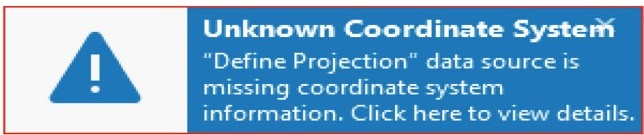
You should get a warning message on the upper right corner that this layer has an unknown coordinate system.
The Unknown Coordinate System means that Salinity.shp has missing spatial reference information. Therefore, Salinity.shp might not be displayed in the extent of lake.tif and GPS.shp. This is because Salinity.shp is missing information about the datum (spatial information), i.e. the software doesn’t know where to place it.
- Using Windows Explorer navigate to your ex10 folder and notice that the shapefile GPS contains one file with the extension “.prj” and notice that Salinity does not contains this file (there is no Salinity.prj).
The prj file contains the “projection information” that all GIS software need to place the data in their correct place. (The raster layer Lake.tif contains a file Lake.tfw that does this function).
- Double click both the GPS.prj file and the Lake.tfw and open them with Notepad and you’ll be able to see their content.
No need to understand them, but know that these are text files with projection information. These are THE ONLY files that can be altered/deleted by humans if we know (or suspect) they’re wrong. No other file should be manipulated with Windows explorer. If necessary (e.g. to rename or move GIS files ALWAYS use the Catalog tool (Catalog Pane) inside Arcgis Pro.
Task 2 – Define projection
The Salinity Layer includes total dissolved solid (TDS) information about the water in the lake. Therefore, it is supposed to be located inside the lake. The reason it is not located there is because it is missing projection information.
Note: Depending on the order that you added the first two layers, Salinity might or might not fit initially in the map screen.
In this step, you will assign a datum to Salinity layer, so it will move automatically into its right location inside the lake.
- Get the Spatial Reference info of Salinity.shp at this moment.
It should say “Unknown Coordinate System” and no more info.
- Click the Analysis tab on the ribbon, in the Geoprocessing group, click the Tool button and click the Toolboxes tab, go to Data Management Tools > Projections and Transformations >Define Projection.
- Input Dataset: Salinity.shp
- Coordinate System: click the drop-down arrow select GPS.shp. It will “import” the information from this layer
- Click Run
When finished, notice that Salinity now shows in the current window. Also check using the Windows Explorer that the .prj file has appeared in the salinity.shp group (you might need to refresh the view in the Explorer for this to s how, press F5).
Note: Notice that Define Projection didn’t create a new dataset (no output file). It didn’t change any of the coordinates. It only wrote a piece of code (like a prj or tfw file) to tell the software what the CURRENT projection is. This tool is used when you know that the projection for a layer is missing or incorrectly recorded. Obviously you should know what the correct projection/coordinate system is when you get some data or create one yourself. Always check for the metadata or data description in the site you’re downloading the data from. (e.g. in MassGIS go to the Spatial reference of MassGIS data page for info).
Task 3 – Changing projections
As mentioned before some functions require that all layers involved have the same coordinate system. Imagine trying to clip a layer with units in degrees (Lat-Long) with a polygon with units in meters (UTM)! This issue is approached differently by different software and by different functions within one software. So, to be safe, all layers that need to “interact” like when we do geoprocessing operations should have the same coordinate system. Also, sometimes, it’s hard to define a buffer for a layer in DD!
The Project tool converts geographic data from one coordinate system to another. Unlike the Define Projection this tool does create a brand new file with new coordinates.
You are now going to project GPS from latitude – longitude onto Universal Transverse Mercator (UTM) zone 15 N.
The raster layer (lake.tif) and vector layer GPS.shp in the Content pane have the same datum (NAD1983) but different coordinate systems. The lake is registered in UTM projection zone 15 N, and the GPS is in geographic coordinates (Lat-long).
- Open the Toolboxes and go to Data Management Tools >Projections and Transformations > Project
- Input: GPS
- Output: GPS_UTM
- Output coordinate system (see below for alternative): click the down arrow and choose Lake.tif to import the configuration of the raster image (NAD_1983_UTM_Zone_15N)
- Geographic Transformation: Leave empty. It’s not necessary as both layers are in the datum NAD83
- Click Run
The GP_UTM layer is in the same coordinate system as Lake.tif
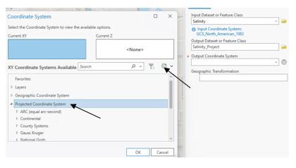
Optional: instead of instruction “c” where we imported the info from an existing layer, if we don’t have a layer to import the parameters for the “Output Coordinate System” you should click the little sphere symbol to the right of the Output box and then expand Projected Coordinate System \UTM \North America \NAD 1983 and select NAD 1983 UTM Zone 15N and click OK. Please try it.
Part 2: Playing with projections in ArcGIS
There are hundreds of projections. Sometimes different maps of the same area look different, some are longer in N-S directions, others longer E-W, sometimes the map looks sort of tilted, etc. You need to get familiar with the characteristics of several projections and/or coordinate systems in order to use the most suitable one for your task. Now we’ll just play a little changing some projections. Your task is to search for the projection that makes the Earth look like a heart.
- Insert a new map in your project and don’t load any dataset, we’ll use the base maps provided
- Zoom out in the map view until you can see the whole world in the screen (it’ll look like a rectangle)
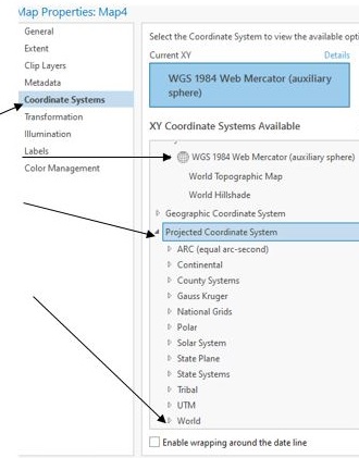
- Get the properties of the Map in the CP and open the Coordinate Systems tab
- Notice that the current coordinate system is WGS 1984 Web Mercator (auxiliary sphere)
- Expand Projected Coordinate System and go to Projected Coordinate Systems – World
- Click on the first projection Adams Square II
- Click the Apply button (to leave the dialog open) and move the dialog to the side to see your map
- Select next Aitoff and so on
- Continue testing different projections. Use only the ones that have “World” in their names. Make sure to try conic, cylindricals, azimuthals, equal areas, equidistants, etc. projections.

Question 5. What is the name of the projection of the world that looks like a heart?
In conclusion different coordinate systems (CRS) serve different purposes. By choosing the correct CRS, you ensure that features on your map are represented accurately. It is important to know the coordinate system of your data! If you need to transform your data to another system, you must know the “starting” system in order to change it. When all the data comes from one source, e.g. MassGIS, everything will have the same system. When data comes from multiple sources they might have different CRS’s and before doing any geoprocessing operation they must be transformed to a common CRS
Part 3: Georeferencing
Raster data are commonly obtained from many sources, such as aerial photographs, satellite images, and scanned maps. Scanned maps and some downloadable images from the internet usually do not contain spatial reference information. Therefore, these images cannot be represented on your map, and their locations will not fit correctly on the surface of the earth. Thus, to use these types of raster data in GIS analysis or as a background image you will need to use accurate location data to align or georeference the raster data to a map coordinate system.
Scenario: You are an ecologist and found on the internet an image representing Silurian aquifer in east Wisconsin. The image has a false coordinate system (arbitrary numbers assigned when scanned), and the rest of your digital data are registered to a geographic coordinate (Latitude – Longitude). To georeference the scanned image, you will use a vector layer of Wisconsin.
Task 1 – Preparing data
- Create a new project or just insert a new map in the previous project. Call the new map Georeferencing.
- Add the dataset State48.shp.
- Select the state Wisconsin and export it into a new shapefile (if saved outside GeoDB) or feature class (if saved inside GeoDB). Call it Wisconsin and add it to the map.
- Turn off or remove State48.shp.
- Symbolize Wisconsin as a hollow polygon with red outline.
- Add to the map the image called WI_Aquifer.jpg. You should get a coordinate system warning like in part 1 task 1.
Question 6. What is WI_Aquifer.jpg current coordinate system?
This aquifer map shows the location of a Silurian age aquifer in the state.
- In the CP right click on WI_Aquifer.jpg and Zoom to layer. Notice where it’s located in relation to the other layers. Also, hover over the image and notice the absurdity of the coordinates shown in the bottom bar.
- Zoom to Wisconsin.
- Turn off the World Topographic Map and World Hillshade because they are not going to be used in the next task. Only keep Wisconsin and WI_Aquifer
Task 2 –Georeference the raster
- In the CP, highlight WI_Aquifer image.
- Click the Imagery tab in the ribbon, in the Alignment group, and click Georeference button to open the Georeference tab.
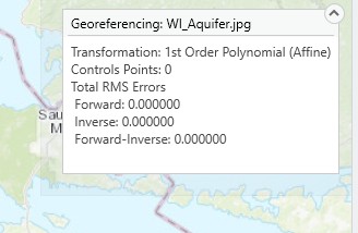
Tools on the Georeference tab are divided into several groups, in order left to right, to help you use the correct tools in the different phases of your georeferencing session. Once you click on the Georeference tab, the top right corner of the Map View, will show the “WI_Aquifer” that will be georeferenced and the RMS, which is empty (Errors), because the georeferencing process hasn’t started yet.

- Make sure that you are zoomed to Wisconsin and in the Prepare group, click Fit to Display.
The raster layer you are georeferencing is placed with the current map display. You can also use the Move, Scale, and Rotate tools in the Prepare group to place the raster as needed and get it as close as possible to its correct position/size (try these tools to practice).
- In the Adjust group, click the Add Control Points tool to create control points. Notice that the cursor changes to a crosshair.
- To add a control point, first find a location easily identifiable on both features (in this case corners of the state). First click on WI_Aquifer (source layer) then click the same location on Wisconsin (target layer) on the map.
If you want to zoom or pan while doing this use the mouse wheel or press the C letter on the keyboard to turn off the “add control point” cursor momentarily.
- Keep adding control points in multiple places around the whole outline of the state until you’ve added like 20 (check the Georeferencing window on the upper right of the map).
Notice how the scanned image adjusts itself to the outline of the state as we add more control points. This process is called Rubbersheeting. Imagine you’re trying to fit/stretch a piece of rubber into a definite shape. Also notice that some points will not fit as well as others, this is OK for now.
- In the Review group, click the Control Point Table button to evaluate the residual error for each control point. Currently you have ~20 control points (it’s OK if you have more or less), and this is sufficient to georeference your image.
- Look at the Forward RMS error in the Georeferencing window in the upper right. This number should be as small as possible.
- Now look at the individual Residuals (error) for each point in the Control Point table. If you find a point has a significantly large value highlight it and delete.
Aim for an error between 0.02 and 0.03 and this is acceptable.
- On the Adjust group, click the drop-down arrow of Transformation , choose the transformation you want to use. The transformation depends on the number of control points. In this exercise, use the 2nd order polynomial if you have more than 6 control points or 3rd order polynomial if more than 10 points.
Observe that as you increase the order of the transformation the error (RMS) decreases and the fit is better (if the points were correct). Also notice that the white area around the scanned map might get all warped and out of shape. This is fine, we don’t care about it.
- When happy with the results push the Save button on the Save group in the ribbon (Georeference tab) then Close Georeference in the same ribbon.
Now your raster is georeferenced and you can now digitize the polygon of the aquifer as you learned in the previous exercise (we’re not doing it now, unless you want to practice. Check Ex 9 part 2 for instructions).
Question 7. What is WI_Aquifer.jpg coordinate system after georeferenced?